
This is a study recently completed by one of my MSc students, Annabelle Rogers, who I co-supervised with Prof Ed February and Glenn Moncrieff. We’re busy writing it up for publication, but here’s a little preview.
The study was inspired by this great paper published by Dr Coert Geldenhuys in 1994, explaining how fire determines the distribution of forests in the Southern Cape. You can also read about it, and get a nice intro to our forests, in this interesting SA Forestry Online article.
The premise of the Geldenhuys study was that certain parts of the landscape are protected from fire due to topographic features interacting with the prevailing winds to create “fire shadows”, where fires will rarely occur. Forests establish and expand in these areas, but are periodically “trimmed back” when severe conditions allow fires to burn into the otherwise non-flammable forest edge.
Our hypothesis, beyond confirming the work by Geldenhuys, was that land cover transformation (e.g. urban expansion) is altering the flow of fire through the landscape and creating new or larger fire shadows.
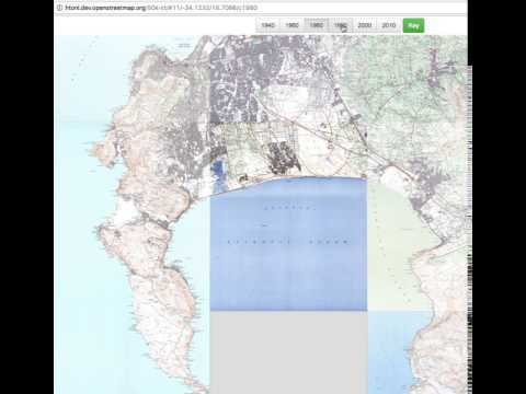
The footprint of the City of Cape Town has expanded quite drastically since the 1940s, providing a good site for this study. Here’s a little Youtube clip I put together using the 1:50 000 topo maps of the City made available by OpenStreetMaps here.
Another advantage is that Zoë Poulsen and Timm Hoffman mapped the change in indigenous forest extent in Table Mountain National Park over the period 1944 to 2008, providing the perfect dataset to validate our models and test our hypothesis.
So, we set Annabelle the task of modelling fire on the Cape Peninsula with and without (i.e. pre-settlement) transformation, to identify areas where the probability of burning may have been affected. This gives us a map of “change in burn probability” and highlights areas that have become fire shadows, which we can compare to the change in forest extent.
I’m not going to go into the details of the fire modelling, including topographic features, developing a fuel model, wind fields and iterations of random ignitions. If you’d like to know more, you’ll have to wait for the paper. Here I present the burn probability maps and quantify the change in burn probability in relation to forest expansion.
First, let’s look at the reduction in burn probabilities when we “disrupt” the fire catchments by making the transformed areas non-flammable. I’ll only present the simple case where we use a homogenous fuel model - i.e. all vegetation burns on the Peninsula in the same way. In reality the vegetation types can differ in flammability quite considerably, especially fynbos vs forest.
Here we present the burn probabilities without transformation, the burn probabilities with transformation, and the difference between the two.
NOTE: I present the code from the R statistical programming language used to do the analysis. Just skip these if you are only interested in the story. I’ve tried to write this so that it makes sense without the code, but include the code for Annabelle and other students interested in performing this kind of analysis. Send me a comment below or email if you feel I haven’t got this right. The code appears in grey boxes, and the output of the code appears either as the images or grey boxes with all lines preceeded by “##”.
library(raster)
library(rgdal)
library(spBayes)
library(rgeos)
library(dplyr)
library(ggplot2)
library(cleangeo)

datwd <- "/Users/jasper/Dropbox/SAEON/Projects/Cape Peninsula/FireShadow/"

#Get and stack files
change <- raster(paste0(datwd,"BP/changeHomog_clip.asc"))
proj4string(change) <- "+proj=utm +zone=34 +south +datum=WGS84 +units=m +no_defs +ellps=WGS84 +towgs84=0,0,0"
transformed <- raster(paste0(datwd,"BP/trans_homog_clip.asc"))
proj4string(transformed) <- "+proj=utm +zone=34 +south +datum=WGS84 +units=m +no_defs +ellps=WGS84 +towgs84=0,0,0"
untransformed <- raster(paste0(datwd,"BP/untrans_homog_clip.asc"))
proj4string(untransformed) <- "+proj=utm +zone=34 +south +datum=WGS84 +units=m +no_defs +ellps=WGS84 +towgs84=0,0,0"
untransformed <- projectRaster(untransformed, transformed)

bp <- stack(untransformed, transformed, change)

par(mfrow=c(1,3))
plot(bp[[1]], main = "Untransformed", col = rev(heat.colors(100)))
plot(bp[[2]], main = "Transformed", col = rev(heat.colors(100)))
plot(bp[[3]], main = "Change (U - T)", col = rev(heat.colors(100)))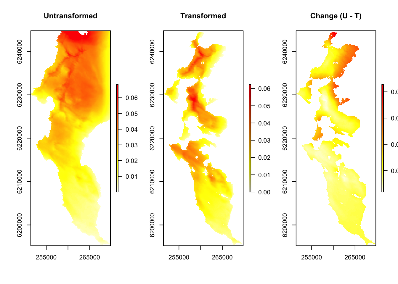
par(mfrow=c(1,1))So higher, “redder” values represent a greater probability of burning, but note that positive values in the “change” layer represent reduced burn probability, because it represents the difference Untransformed - Transformed. Also note that the funny numbers around the border are metres from the South Pole (y-axis) and from the Greenwich Meridian (x-axis), because the data are projected with the UTM 34S coordinate reference system.
Where’s your house?
Now let’s get the forest change layers from Poulsen and Hoffman 2015 and plot forest change around Table Mountain.
f1944 <- readOGR(paste0(datwd, "forest/forestUTM1944.shp"), "forestUTM1944") #Get the layers## OGR data source with driver: ESRI Shapefile
## Source: "/Users/jasper/Dropbox/SAEON/Projects/Cape Peninsula/FireShadow/forest/forestUTM1944.shp", layer: "forestUTM1944"
## with 224 features
## It has 7 fieldsf2008 <- readOGR(paste0(datwd, "forest/forestUTM2008.shp"), "forestUTM2008")## OGR data source with driver: ESRI Shapefile
## Source: "/Users/jasper/Dropbox/SAEON/Projects/Cape Peninsula/FireShadow/forest/forestUTM2008.shp", layer: "forestUTM2008"
## with 205 features
## It has 15 fields###Ignore this code for now. It's a nicer way of plotting the map, but...
# f2008[205,] #Orangekloof polygon needs fixing!!!
# f1944@data$id = rownames(f1944@data)
# f1944=gUnionCascaded(f1944,id=f1944$id)%>%
# gSimplify(0.001,topologyPreserve = T) #Fix topology issues
#
# f2008@data$id = rownames(f2008@data)
# f2008=gUnionCascaded(f2008,id=f2008$id)%>%
# gSimplify(0.001,topologyPreserve = T) #Fix topology issues
# map <- ggplot(f2008) +
# aes(long, lat, group = group, fill = "#4393C3") +
# geom_polygon(alpha = 0.5) +
# coord_equal() +
# theme(legend.position="none")
sf1944 <- crop(f1944, extent(255000, 270000, 6230000, 6240000))
#sf2008 <- crop(f2008, extent(255000, 270000, 6230000, 6240000))
plot(sf1944, col = "forestgreen", border = "white")
plot(f2008, add = T, col = "green", border = "white")
plot(f1944, add = T, col = "forestgreen")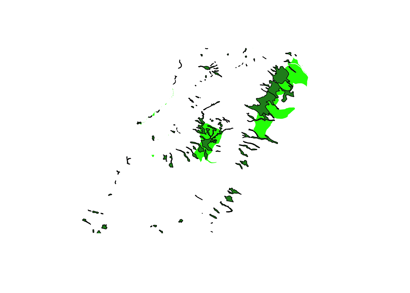
Here the dark green is the forest extent in 1944, while the light green indicates the additional forest extent in 2008 - lots of expansion!
Now I’d like to overlay the burn probabilities with the areas that were “stable fynbos” vs “stable forest” vs “forest expansion” over the 1944 to 2008 period and show you the difference as boxplots, but to work with them we’ll need them as raster data (i.e. gridded as opposed to polygons). So first I rasterize each layer to a 90m grid and plot fynbos (0 - grey), stable forest (2 - green) and areas of forest expansion (1 - yellow). Please ignore the confusing scale bar.
fr1944 <- rasterize(f1944, bp, fun = "count", field = 1, background = 0) #create a raster with "1" where forest occurred
fr2008 <- rasterize(f2008, bp, fun = "count", field = 1, background = 0) #create a raster with "1" where forest occurred

frDelta <- fr2008 + fr1944

plot(crop(frDelta, extent(255000, 270000, 6230000, 6240000)))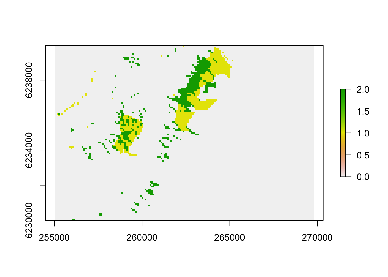
Now we can extract them into one dataframe (i.e. a table of data) and bin them into vegetation change classes…
dat <- as.data.frame(na.omit(rasterToPoints(stack(bp, frDelta))))

dat$layer[which(dat$layer == 0)] <- "Stable Fynbos"
dat$layer[which(dat$layer == 1)] <- "Forest Gain"
dat$layer[which(dat$layer %in% c(2,3))] <- "Stable Forest" #Note there is some erroneous overlap in the 2008 polygons

dat$layer <- as.factor(dat$layer)

#write.csv(dat, "/Users/jasper/Dropbox/SAEON/Projects/Cape Peninsula/FireShadow/spBayes/data.csv")

head(dat)
## x y untrans_homog_clip trans_homog_clip changeHomog_clip
## 1 259845 6244515 0.066660 0.009665 0.056995
## 2 259935 6244515 0.066940 0.008860 0.058080
## 3 260025 6244515 0.067385 0.008220 0.059165
## 4 260115 6244515 0.067505 0.007085 0.060420
## 5 259665 6244425 0.063040 0.010975 0.052065
## 6 259755 6244425 0.063715 0.010565 0.053150
## layer
## 1 Stable Fynbos
## 2 Stable Fynbos
## 3 Stable Fynbos
## 4 Stable Fynbos
## 5 Stable Fynbos
## 6 Stable FynbosSo there’s the top few lines of the table above. Now we use these data to draw a box and whisker plot of the reduction in burn probability by class. Here the horizontal mid-line represents the midpoint of the observed values for each class (the median), the box represents the upper and lower quartiles (i.e. 50% of the records for each class fall inside the box), the “whiskers” represent ~75% of the data in each class, and the points (i.e. the black smudge above “Stable Fynbos”) represent outliers that are further from the rest of the data than we would expect.
g <- ggplot(dat)
g <- g + stat_boxplot(aes(y = changeHomog_clip, x = layer, group = layer), position = "dodge") +
  ylab("Reduction in burn probability") +
  xlab("Vegetation Change")
g #to plot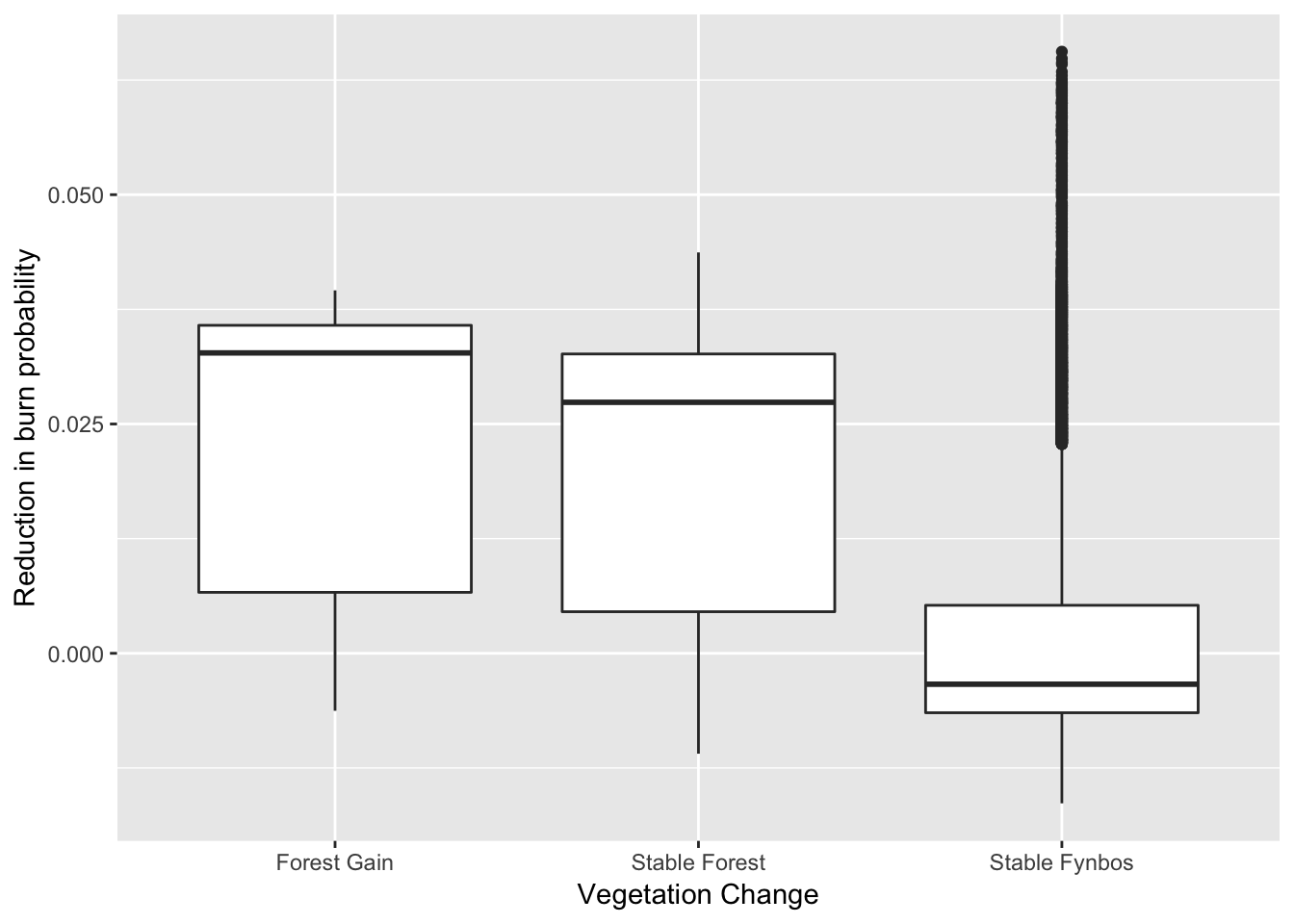
That “Forest Gain” and “Stable Forest” have much higher medians and “boxes” clearly indicates that forest has remained stable and/or expanded in the areas where there has been a reduction in burn probability. There are many possible reasons for the “outliers” in the “Stable Fynbos” class, but the two main reasons are likely to be that a) not all fynbos sites that have suffered a reduction in burn probability are able to sustain forest (e.g. too dry), and b) these sites may well be transitioning to forest, but more time is needed for them to do so.
While this plot looks very convincing, unfortunately it would never fool journal reviewer number three…

They’ll argue there’s spatial autocorrelation (i.e. things that are close in space are likely to be similar anyway) and will want to see some fancy spatially explicit statistics that don’t tell you any more than this boxplot.
So here are some convolutedly fancy stats for those of you who are interested. Skip to the brief discussion at the end if you’re not interested in the stats :)
We’ll start by thinning the data a little by subsampling. Running a spatially explicit Bayesian model on the ~34000 data points (i.e. 90m grid cells) we have requires a very very big computer, and this is just a blog post. Let’s try 10% of the data and plot it to check that it’s representative of the full dataset (as plotted above).
set.seed(1) #Pick a string of random numbers so that we can replicate the sampling

sdat <- dat[sample(1:nrow(dat), nrow(dat)/10),] #Take a 10% sample

g <- ggplot(sdat)
g <- g + stat_boxplot(aes(y = changeHomog_clip, x = layer, group = layer), position = "dodge") +
  ylab("Reduction in burn probability") +
  xlab("Vegetation Change Class")
g #Plot the sample to see if it is representative of the whole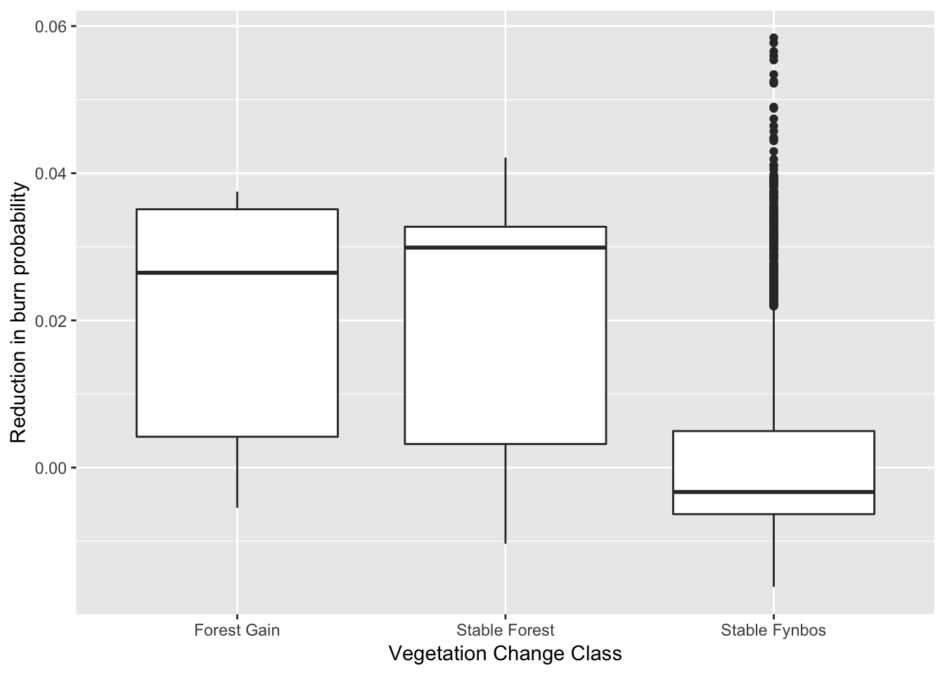
Looks pretty representative.
It turns out it takes ~12 hours to run the following code on the 10% subset of the data on a x86_64-apple-darwin13.4.0 MacBook Pro (so I’ve commented out the next code chunk so I don’t have to run it each time I compile this blog post). I think we’ll need to run the full dataset on a cluster…
Skip this section if you’re more interested in the results.
# ### Set up a convolutedly long set of model inputs which I won't eplain
# B <- as.matrix(c(1:3))
# p <- length(B)
#
# sigma.sq <- 2
# tau.sq <- 0.1
# phi <- 3/0.5
#
# n.samples <- 2000
#
# starting <- list("phi"=3/0.5, "sigma.sq"=50, "tau.sq"=1)
#
# tuning <- list("phi"=0.1, "sigma.sq"=0.1, "tau.sq"=0.1)
#
# ### Set up 2 sets of different "prior beliefs" to see how much this affects the model - note that I've just gone with some simple ones here and should really explore a bigger range
# priors.1 <- list("beta.Norm"=list(rep(0,p), diag(1000,p)),
#                  "phi.Unif"=c(3/1, 3/0.1), "sigma.sq.IG"=c(2, 2),
#                  "tau.sq.IG"=c(2, 0.1))
#
# priors.2 <- list("beta.Flat", "phi.Unif"=c(3/1, 3/0.1),
#                  "sigma.sq.IG"=c(2, 2), "tau.sq.IG"=c(2, 0.1))
#
# ### Choose a model for the spatial autocorrelation
# cov.model <- "exponential" #A very rapid decay model. This should be fair for our data, but I'll need to play with this for publication
#
# n.report <- 500
# verbose <- TRUE
#
# ###Run the models
# m.1 <- spLM(changeHomog_clip~layer, coords=as.matrix(sdat[,1:2]),
#             data = sdat, starting=starting,
#             tuning=tuning, priors=priors.1, cov.model=cov.model,
#             n.samples=n.samples, verbose=verbose, n.report=n.report)
#
# m.2 <- spLM(changeHomog_clip~layer, coords=as.matrix(sdat[,1:2]),
#             data = sdat, starting=starting,
#             tuning=tuning, priors=priors.2, cov.model=cov.model,
#             n.samples=n.samples, verbose=verbose, n.report=n.report)
#
# burn.in <- 0.5*n.samples
#
# ###Recover beta and spatial random effects
# m.1 <- spRecover(m.1, start=burn.in, verbose=FALSE)
# m.2 <- spRecover(m.2, start=burn.in, verbose=FALSE)
#
# round(summary(m.1$p.theta.recover.samples)$quantiles[,c(3,1,5)],2)
# round(summary(m.2$p.theta.recover.samples)$quantiles[,c(3,1,5)],2)
#
# round(summary(m.1$p.beta.recover.samples)$quantiles[,c(3,1,5)],2)
# round(summary(m.2$p.beta.recover.samples)$quantiles[,c(3,1,5)],2)
#
# m.1.w.summary <- summary(mcmc(t(m.1$p.w.recover.samples)))$quantiles[,c(3,1,5)]
# m.2.w.summary <- summary(mcmc(t(m.2$p.w.recover.samples)))$quantiles[,c(3,1,5)]
#
# save(m.1, paste0(datwd, "model1.RData"))
Here’s one I prepared earlier ;)
load(paste0(datwd, "model1.RData")) #Get previously run model output

#round(summary(m.1$p.theta.recover.samples)$quantiles,2) #If you're running this code this gives you the spatial autocorrelation estimates

round(summary(m.1$p.beta.recover.samples)$quantiles,3)
## 2.5% 25% 50% 75% 97.5%
## (Intercept) 0.009 0.016 0.020 0.024 0.032
## layerStable Forest -0.015 -0.005 0.000 0.004 0.013
## layerStable Fynbos -0.031 -0.023 -0.019 -0.015 -0.008So this gives us the median (50%) and quantiles (0.025, 0.25, 0.75, 0.975) of the posterior probability distributions of the estimated average values for each class. “Forest Gain” is the intercept, which is all positive (i.e. lower probability of burning), and overlaps with “Stable Forest”, but does not overlap with “Stable Fynbos”, which confirms what we knew already! Although it’s a little difficult to interpret. Let’s try a boxplot to illustrate this more clearly.
x <- as.data.frame(round(summary(m.1$p.beta.recover.samples)$quantiles,3))

rownames(x) <- levels(sdat$layer)
colnames(x) <- c("min", "lower", "mid", "upper", "max")

#m.1.w.summary <- summary(mcmc(t(m.1$p.w.recover.samples)))$quantiles[,c(3,1,5)]

Pa <-  ggplot(x,aes(rownames(x))) +
  geom_boxplot(aes(ymin=min,lower=lower,middle=mid,upper=upper,ymax=max),
              stat="identity") +
   ylab("Reduction in burn probability") + xlab("Vegetation Change Class")

Pa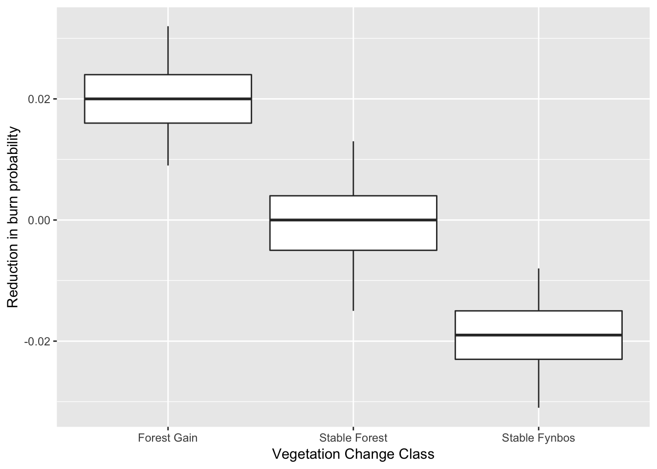
So the forest expanded at sites where the probability of burning has been reduced, because land cover transformation has created new “fire shadows”. Null hypothesis accepted?
Note that there are a bunch of assumptions etc that I haven’t included here. E.g. having more people usually increases ignitions, resulting in more fires. This may also have a biased spatial pattern, like fires are most likely to start along the wildland-urban interface, etc.
Either way, I think there are many reasons why this analysis is interesting despite it’s flaws, and I suspect the story is at least partially true. The real question is how can we manage this? Do we allow these areas to succeed to forest, despite the loss of fynbos biodiversity at these sites? And the risk of catestrophically big fires if a fire is started in the ~50-100 year period while the fynbos is being invaded by forest and is incredibly flammable?
For the reviewer #3’s among you - here are the model diagnostics:
plot(m.1$p.beta.recover.samples)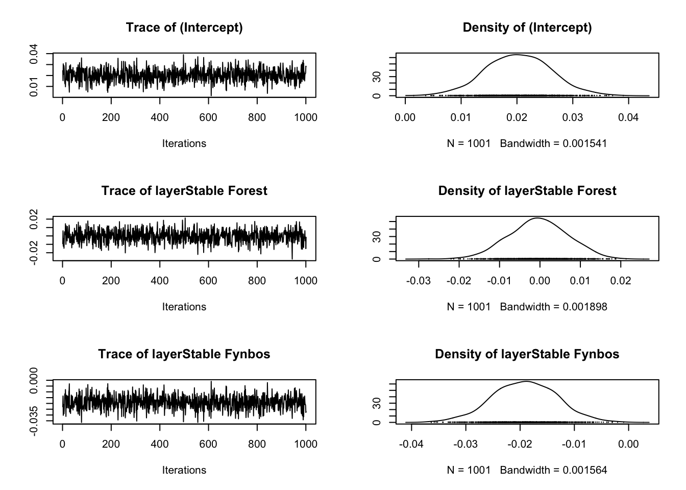
It looks like the model converged nicely :)
And the session info:
sessionInfo()## R version 3.5.1 (2018-07-02)
## Platform: x86_64-apple-darwin15.6.0 (64-bit)
## Running under: macOS High Sierra 10.13.6
##
## Matrix products: default
## BLAS: /Library/Frameworks/R.framework/Versions/3.5/Resources/lib/libRblas.0.dylib
## LAPACK: /Library/Frameworks/R.framework/Versions/3.5/Resources/lib/libRlapack.dylib
##
## locale:
## [1] en_GB.UTF-8/en_GB.UTF-8/en_GB.UTF-8/C/en_GB.UTF-8/en_GB.UTF-8
##
## attached base packages:
## [1] stats graphics grDevices utils datasets methods base
##
## other attached packages:
## [1] cleangeo_0.2-2 maptools_0.9-3 ggplot2_3.0.0 dplyr_0.7.6
## [5] rgeos_0.3-28 spBayes_0.4-1 Formula_1.2-3 magic_1.5-8
## [9] abind_1.4-5 coda_0.19-1 rgdal_1.3-4 raster_2.6-7
## [13] sp_1.3-1
##
## loaded via a namespace (and not attached):
## [1] Rcpp_0.12.18 plyr_1.8.4 compiler_3.5.1 pillar_1.3.0
## [5] bindr_0.1.1 tools_3.5.1 digest_0.6.15 gtable_0.2.0
## [9] evaluate_0.11 tibble_1.4.2 lattice_0.20-35 pkgconfig_2.0.1
## [13] rlang_0.2.1 yaml_2.2.0 blogdown_0.8 xfun_0.3
## [17] bindrcpp_0.2.2 withr_2.1.2 stringr_1.3.1 knitr_1.20
## [21] rprojroot_1.3-2 grid_3.5.1 tidyselect_0.2.4 glue_1.3.0
## [25] R6_2.2.2 foreign_0.8-71 rmarkdown_1.10 bookdown_0.7
## [29] purrr_0.2.5 magrittr_1.5 scales_0.5.0 backports_1.1.2
## [33] htmltools_0.3.6 assertthat_0.2.0 colorspace_1.3-2 labeling_0.3
## [37] stringi_1.2.4 lazyeval_0.2.1 munsell_0.5.0 crayon_1.3.4