4 Tidy Data
This section is aimed at helping you develop a relatively simple reproducible workflow for your project (i.e. Deliverable 2 described in section 1.3\(^*\)) and providing a demonstration of some of the Tidyverse tools for wrangling and tidying your data.
\(^*\)But note that the content of the previous 2 sections are important for the deliverable too.
Ultimately, tidying your data is the first step in your data analysis and communication workflow.
But first you need to get your data into a digital format…
4.1 Data entry
NOTE: This section may not be relevant to the module deliverable, because you should have an example dataset that’s already in digital format, but it will be useful if/when you collect new data of your own.
Before we start, I should highlight that one very good way of reducing errors in data entry and improving quality assurance and quality control (QA/QC) is to make use of various forms of data validation like drop down lists and conditional formatting. These can be used to limit data types (i.e. avoids you entering text into a numeric column or vice versa), or limiting the range of values entered (e.g. 0 to 100 for percentages), or just highlighting values that are possible, but rare, and should be double-checked, like 100m tall trees. Unit errors are incredibly common in ecological data entry, especially for things like plant height where you may be measuring 20cm tall grasses and 20m tall trees!!! Drop down lists really come into their own when you’re working with lots of different Latin species names etc. Typos, spelling errors and synonyms can take weeks of work to fix! Restricting the names to a drop-down list from a known published taxonomic resource really makes a huge difference!
Here’s an example from a vegetation survey practical I ran as part of the BIO3018F Ecology and Evolution 3rd-year field course. If you go to the Sites sheet, you’ll see that the first two columns Site and Point are drop-down lists that reference the RangeLimits spreadsheet, to make entry easy and to prevent spelling mistakes etc. You’ll also notice that the different columns have specified ranges, and that a number outside the range is entered (e.g. anything >100 for PercentBareSoil) then the cell is highlighted with a warning. You can see the data validation rules by selecting a cell in the column of interest and clicking Data > Data validation
It’s often easy to forget to collect some measurements etc when in the field, like site-level information. Sometimes what I do to prevent this is set up the next data entry sheet (trait data in this case), to require that you fill in the site name from a drop-down list that is populated in the site data sheet. This limits the names you can use to only those that have site data, and serves as a reminder should you have forgotten. Check out the SitePoint column in the Traits sheet.
I’m not going to go into how to do data validation in spreadsheets, but here are links for:
I’m sure there are plenty of other online resources too.
One thing I really like about Google Sheets is that you can set your sheet to work in “offline mode” on your phone or tablet, which allows you to do data entry directly into the sheet in the field, which then syncs to your Google Drive when you go back online (I’d imagine you can do the same with MS Excel and One Drive, but I’ve never tried it). This really saves time (and errors) on entering written field data sheets into a spreadsheet later, and allows you to take advantage of the data validation rules in the field, which are harder to set up with pen or pencil… The only issue is that if you make a typo etc that isn’t caught by the data validation you’re likely to be stuck with it…
Take lots of photos (preferably geotagged)!!! It often helps you identify and fix errors later, and is great for getting context for your data or for working out why some sites have weird values etc.
4.2 Reproducibility - start as you mean to finish
Now that you have your data, the temptation is to open an R script and get analyzing, or worse yet, open your raw data file in a spreadsheeting programme and crack out a few simple graphs… WAIT!!!
Never do data analyses in your raw data files!!! These are your raw data, and they should stay that way. In fact, they should be set to be read-only so that you can’t edit them even if you wanted to. If you were to edit these files directly and make a mistake, like say sort a column without sorting the rest of the table, that’s it! Alles is kaput! You need your raw data files so that you have somewhere to look when you suspect you’ve done something bad to your data.
Beyond data management, there’s code management, and version control software like GitHub is your friend, providing a backup of all your scripts, versioning (i.e. a record of changes of your scripts that you can revert should you need to - i.e. no more scripts named “analysis_final_final_FINAL.R”) and is a great tool for collaboration and sharing. In fact, GitHub can manage much more than just code, and can host your manuscript, output figures and tables, and even small datasets. Here’s a quick start guide for GitHub that shows you the basic functionality in ~10 minutes. I highly recommend working through it before you move on to the next steps…
The trick to reproducible research is to start as you mean to finish. By this I mean that it is much easier to produce a reproducible research workflow if you work reproducibly from the start, rather than retrofitting a bunch of data and code you’ve already analyzed. This also means that you can reap the benefits of reproducibility during your project, which includes things like easier finding and fixing of errors, easier collaboration, simple splitting of the workflow if you decide that the project could lead to multiple publications, etc.
The next 2 sections are covered in the quick start guide you should have worked through, but I add a few specific comments, and are essentially what you need to do to get set up with a GitHub repo before you get coding.
4.2.1 Creating a Git repository (or repo for short)
- Go to your online GitHub account (e.g. https://github.com/jslingsby)
- Click on the
+in the top-right and selectNew repository - Give your repository a name and description
- Choose whether you want the repo to be public or private (e.g. if you’re going to include sensitive data or otherwise don’t want the world to see what you’re doing)
- I usually
Add a READMEfile, that allows you to write a description of the project, explain the contents of the repo, etc - I also usually
Add .gitignoreand chooseRfrom the templates. This is a file that allows you to list files and folders that you don’t want GitHub to sync
- e.g. you may want to have a “bigdata” folder on your local machine with files too large to sync to GitHub (~>50MB), although check out Git Large File Storage, or an “output” folder with large figures etc that you can easily reproduce from the code
- Add a license if you want too
- Click
Create repository
4.2.2 Cloning your repo to your local machine
- Open RStudio on your laptop (you should already have RStudio and GitHub set up as per the instructions in section 1.4)
- Copy the URL to the repo you just created (e.g. https://github.com/jslingsby/demo)
- In RStudio:
- in the top-right of the window you’ll see
Project: (None)- click on it and selectNew ProjectthenVersion ControlthenGit - In the
Repository URl:box paste the URL to your repo Project directory nameshould fill automatically- For
Create project as subdirectory of:hitBrowseand navigate through your file system to where you want to put your folder for storing your Git repositories. I recommend something like~Documents/GIT(If you’ve used Git before you may have set this already and can skip this step) - Click
Create Repository
You should now see the name of your project/repo in the top-right corner of RStudio where previously you saw Project: (None) and you’re good to go.
Now that you’re working on your local machine you need to set up a folder structure for code, output, data etc (using RStudio or your file explorer). Then you can open an R script, or better yet, an RMarkdown or (better yet) Quarto document that allows you to write text and embed code and images etc.
4.2.3 Keeping your online Git repository in sync
Once you’ve added some content to your project (the local version of the Git repository), you want to sync it back to the online repository…
- From the “Git” tab (top-right window in RStudio), click the check boxes next to the files and folders you’ve created. This is equivalent to git add if you were doing this command line in bash or terminal.
- Click
Commit, enter a log message (notes to yourself or collaborators about what you’re adding), and clickCommitagain. This is equivalent to git commit in command line. - Now you’re going to “push” the changes to the online repository, but first, it’s always good practice to “pull” any changes from the repository to your local machine first. You do this, because if it was a collaborative project, others may have made changes since you last “pulled”. You may also have made changes to the repo directly in the website… To “pull” changes into RStudio, click the green down arrow (next to “Commit”). If it says “Already up-to-date” you can then “push” your changes up to Github by clicking on the green up arrow. This is equivalent to git push.
4.3 Tidy data and data wrangling
Now you’re finally ready to start interrogating your data! But the raw data probably aren’t in a particularly analysis-friendly format, so you need to start with some data tidying and wrangling. You could do this “manually” in a new, appropriately named, copy of your raw data spreadsheet, but then you may not be able to track the changes you’ve made and errors may creep in. Where possible, it’s best to do this step with code. Most of my projects start with a “00_data_cleaning.R” script or similar to read the raw data and create an analysis-ready dataset. If this script takes a long time to run, I may output a new “clean data” file (or files) so that I don’t need to rerun the script every time.
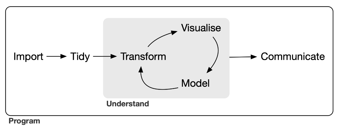
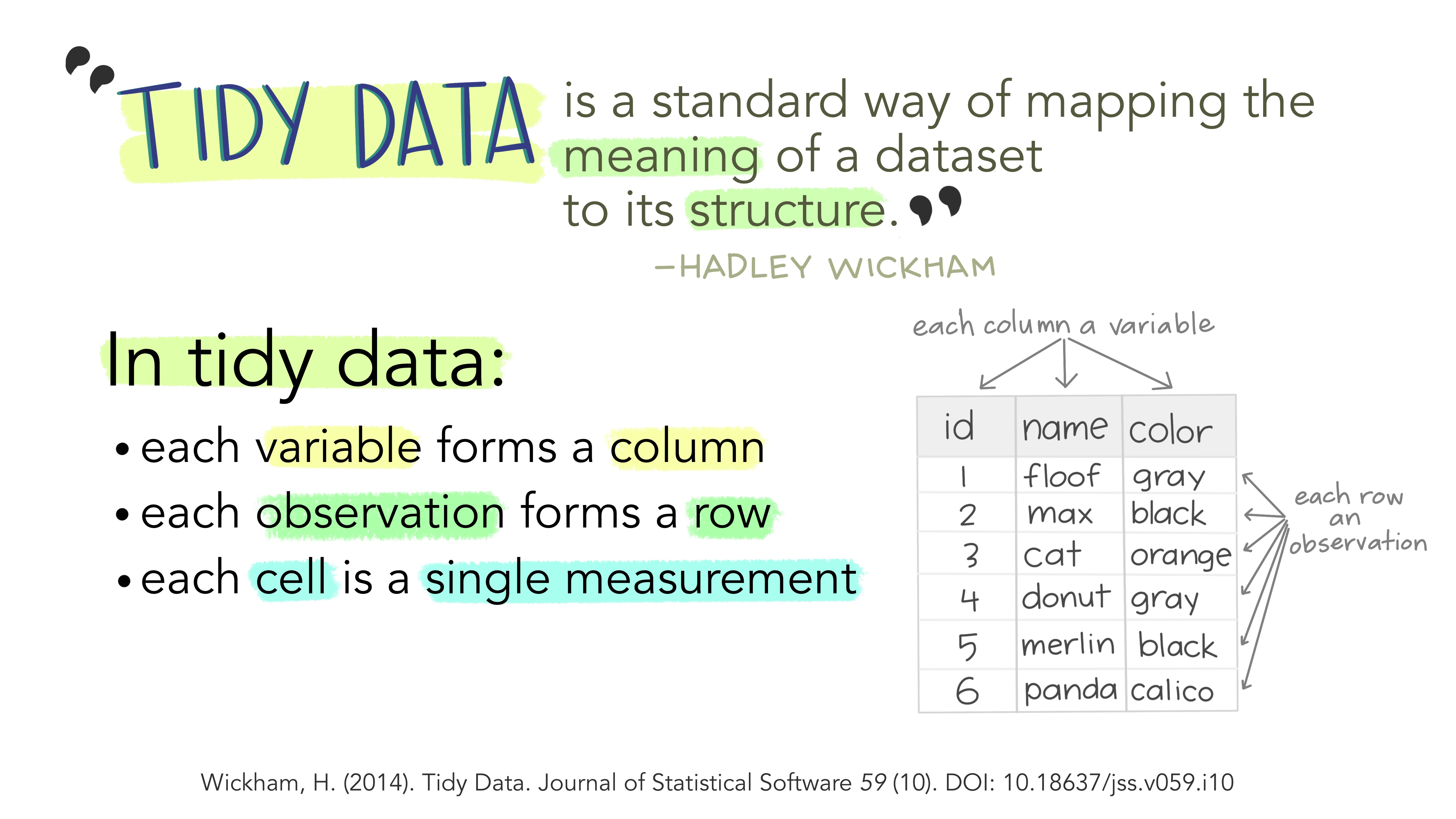
What is tidy data? I strongly recommend you read this short paper on how to keep your data Tidy (Wickham 2014). Following these principles will make life much easier for you once you get to the analysis step…
Here’s the basic idea in nice illustrations by @allison_horst:
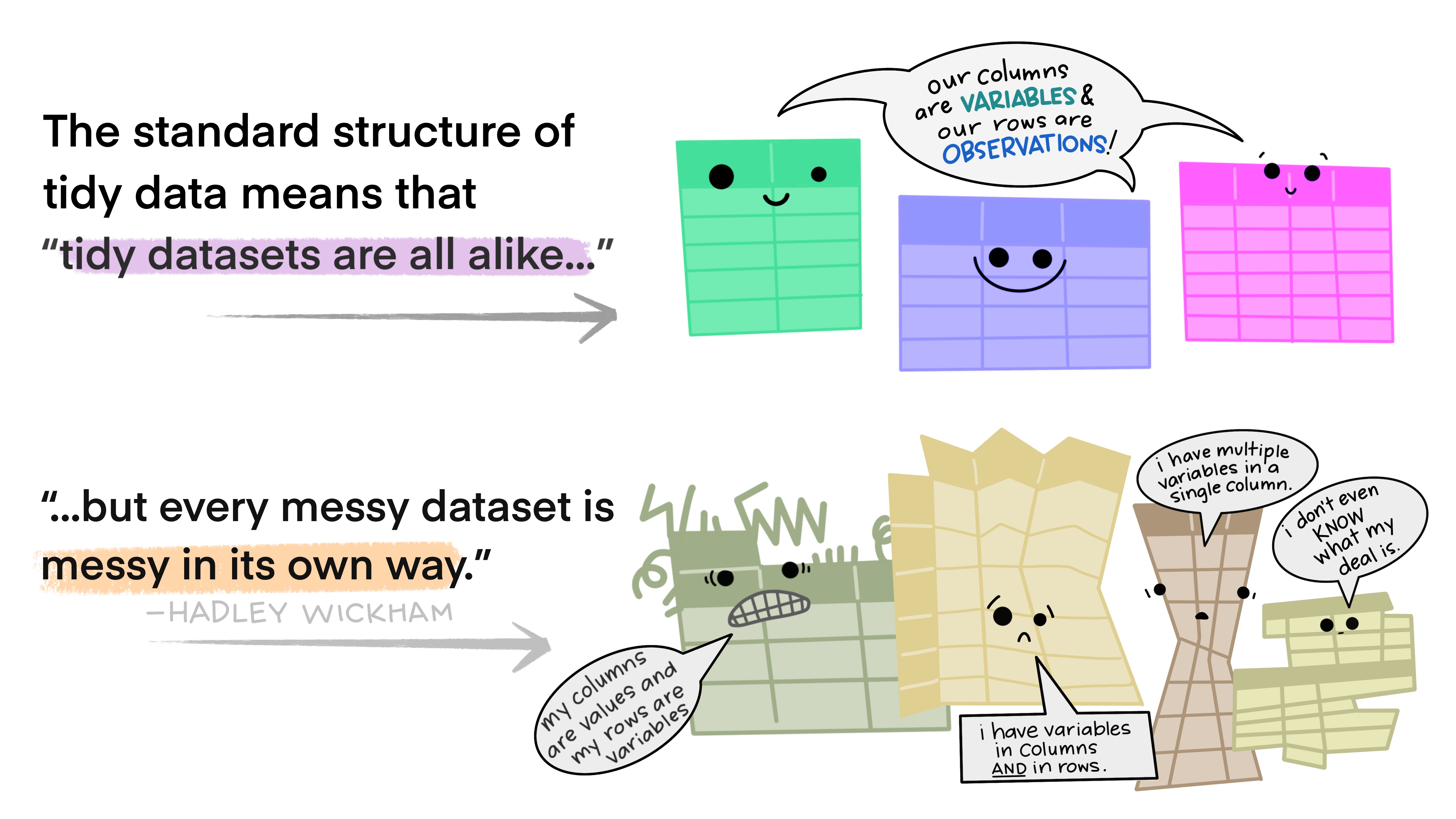
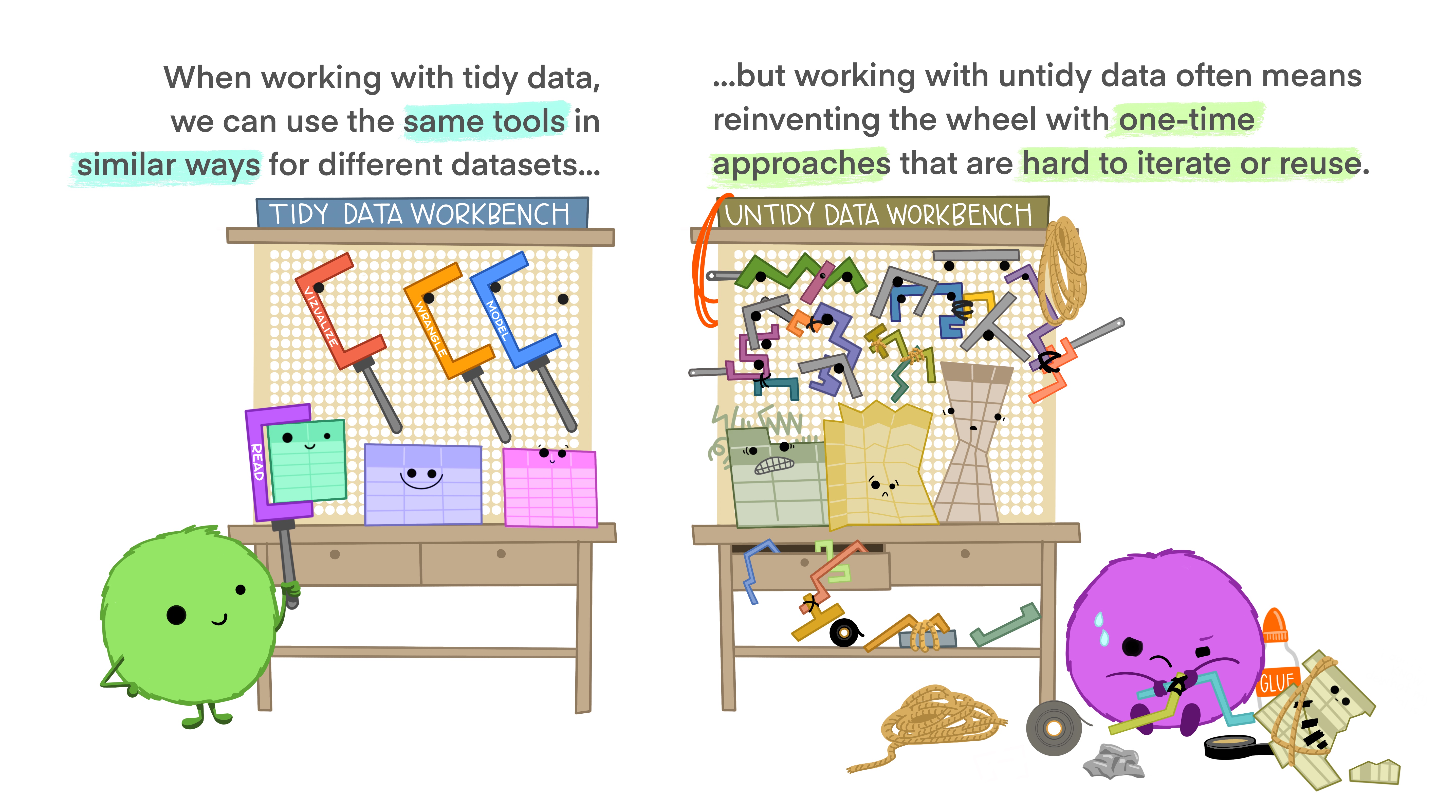
These figures, and the readings for the course, highlight that there are many reasons why you should keep your data in tidy format (Wickham 2014). Unfortunately, as my spreadsheet above demonstrates, it’s not always convenient to enter your data in tidy format, so you inevitably end out needing to do post-entry data formatting. A major problem here is that doing the reformatting manually creates opportunities for introducing errors. This is where it’s a major advantage if you know how to wrangle your data in a coding language like R or Python. This is not to say that coded data wrangling cannot introduce errors!!! You should always do sanity checks!!! But I’d suspect that most of the errors you can make with code will be very obvious, because the outcome is usually spectacularly different to the input.
The rest of this chapter provides a demonstration of some of the functionality of the tidyverse set of R packages, and some of the more common data wrangling errors made in R.
4.3.1 The dataset
This tutorial relies on the BIO3018F prac data mentioned previously. See here if you’d like more details about the data and practical.
4.3.2 The motivation…
Here’s a cool trick. Don’t freak out that I haven’t commented the code with explanations. We’ll break this down in the following sections.
## ── Attaching core tidyverse packages ──────────────────────── tidyverse 2.0.0 ──
## ✔ dplyr     1.1.4     ✔ readr     2.1.5
## ✔ forcats   1.0.0     ✔ stringr   1.5.1
## ✔ ggplot2   3.5.1     ✔ tibble    3.2.1
## ✔ lubridate 1.9.3     ✔ tidyr     1.3.1
## ✔ purrr     1.0.2
## ── Conflicts ────────────────────────────────────────── tidyverse_conflicts() ──
## ✖ dplyr::filter() masks stats::filter()
## ✖ dplyr::lag()    masks stats::lag()
## ℹ Use the conflicted package (<http://conflicted.r-lib.org/>) to force all conflicts to become errorslibrary(readxl)
read_xlsx("data/pracdatasheet.xlsx", sheet = "Sites") %>%
mutate(CanopyCover = 100 - 4.16*Densiometer) %>%
select(!c("SoilColour", "Densiometer")) %>%
pivot_longer(cols = c("PercentBareSoil", "SoilPH", "Dung", "CanopyCover"),
names_to = "variable", values_to = "value") %>%
ggplot() +
geom_boxplot(aes(y = value, x = Site)) +
theme(axis.text.x = element_text(angle = 45, hjust = 1)) +
facet_wrap(vars(variable), scales = "free")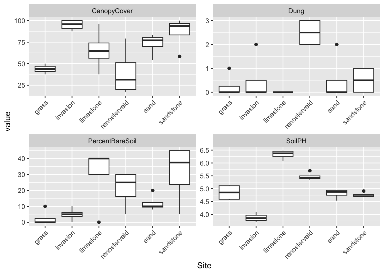
In just 9 lines of code (and it could be fewer if I was being less neat) I read in the raw data with read_xlsx, created a new column that’s a transformation of an existing one with mutate, dropped unwanted variables with select (I didn’t actually need to do this, I was just showing off…), reshaped the entire dataframe from wide format (not tidy) to long format (tidy) with pivot_longer and made a pretty boxplot (ggplot + geom_boxplot) with rotated x-axis text (theme) and separate facets for each environmental variable (facet_wrap).
You too can have these superhero powers!
The rest of this chapter is focused on reading in data and various tricks to wrangle it into different formats, join separate tables, etc. Plotting you will have to learn yourself, but I may show a few simple examples.
4.4 Reading in data
R has a number of different packages to read in data, and there’s even a few that work with different tabular data types just within the tidyverse. These include:
- readr for text files with values separated with tab, comma, or some other delimiter (.txt, .csv, .tsv file extensions)
- readxl for Microsoft Excel files (.xls or .xlsx)
- googlesheets4 for reading data directly from a Google Sheet
There’s others too that can scrape data from web pages, interact with web APIs, or query local or online databases.
Fortunately, within the tidyverse, similar syntax can be used across most data import packages. Check out the cheat sheet.
4.4.1 Read Google Sheets with googlesheets4
Since I gave you the link to a Google Sheet above, you should be able to read the data directly into R using that URL with the googlesheets4 package. Note that it may ask you to authenticate your Google account. You can do this with your personal or UCT account.
# First let's call the libraries with the functions we want to use
library(tidyverse)
library(googlesheets4) # while googlesheets4 is part of the tidyverse, and installed when you install the tidyverse, it isn't a core package, so you have to call it separately

# You may need to tell Googlesheets what account to use (of your own) using the function gs4_auth(), e.g. gs4_auth(email = "myemail@gmail.com"), but in this case we can just tell it not to authenticate as the Google Sheet is publicly accessible
gs4_deauth()

# Now let's have a look at the names of the worksheets (tabs) within the spreadsheet
sheet_names("https://docs.google.com/spreadsheets/d/1U9yNaJFyd6kb5vlKzHhcgM6sLEzw_xVtQxewpH7k0Ho/edit?usp=sharing")
## [1] "Sites" "Traits" "Species" "RangeLimits" "RangeSpecies"Sometimes it shows lots of garble about the online authentication, but finally it shows us that there are five worksheets in the spreadsheet.
Let’s read in the “Sites” sheet and call it edat for “environmental data”, and then print a summary.
WARNING - running the name of a data object in R is usually a bad idea. It typically then shows you every value in the dataset, which can be hundreds of thousands of values! Tidyverse packages just show you a summary and the first few rows of data, which is nice…
edat <- read_sheet("https://docs.google.com/spreadsheets/d/1U9yNaJFyd6kb5vlKzHhcgM6sLEzw_xVtQxewpH7k0Ho/edit?usp=sharing", sheet = "Sites") # read in data## ✔ Reading from "pracdatasheet".## ✔ Range ''Sites''.## # A tibble: 24 × 8
## Site Point SitePoint PercentBareSoil SoilPH SoilColour Dung Densiometer
## <chr> <chr> <chr> <dbl> <dbl> <chr> <dbl> <dbl>
## 1 grass SE grass_SE 0 4.6 7.5YR3/2 0 15
## 2 renoster… SE renoster… 5 5.4 10YR3/2 3 14
## 3 invasion SE invasion… 0 3.79 10YR2/1 0 0
## 4 sand SE sand_SE 10 4.82 10YR6/4 0 5
## 5 sandstone SE sandston… 5 4.91 10YR3/2 0 2
## 6 limestone SE limeston… 0 6.48 10YR2/1 0 9
## 7 grass NE grass_NE 0 5.13 10YR2/2 0 13
## 8 renoster… NE renoster… 30 5.7 7.5YR4/3 2 20
## 9 invasion NE invasion… 5 3.7 10YR5/1 0 0
## 10 sand NE sand_NE 8 4.54 10YR4/3 0 4
## # ℹ 14 more rowsNote that you can also create and write to a Google Sheet with gs4_create() and write_sheet()
4.4.2 Downloading Google Sheets with R
If your spreadsheet is large, reading them into R from online Google Sheets can be slow. In this case you may want to download them as local MS Excel (.xlsx) files. Fortunately, even the download step can be scripted in R with functions from library(googledrive).
##
## Attaching package: 'googledrive'## The following objects are masked from 'package:googlesheets4':
##
## request_generate, request_makedrive_deauth() # Or specify your email with drive_auth(email = "jenny@example.com")
drive_download(file = "https://docs.google.com/spreadsheets/d/1U9yNaJFyd6kb5vlKzHhcgM6sLEzw_xVtQxewpH7k0Ho/edit?usp=sharing",
path = "data/pracdatasheet.xlsx", overwrite = TRUE)## File downloaded:## • 'pracdatasheet' <id: 1U9yNaJFyd6kb5vlKzHhcgM6sLEzw_xVtQxewpH7k0Ho>## Saved locally as:## • 'data/pracdatasheet.xlsx'4.4.3 Read Microsoft Excel files with readxl
Reading data in directly from Google Sheets can be super handy, but it requires an internet connection, and can become quite slow if your dataset gets big. In that case, it’s very easy to download Google Sheets as Microsoft Excel files and read them in using functions in the readxl package.
First, we may want to know what files are in our data folder, which we can do with the base R function list.files(). Note that this function can be very handy if you have lots of files to process, like photos, etc.
NOTE: you need to replace the working directory folder path (“data” here) with wherever you put the data on your computer. In my case, “data” is a folder in the git repo (and thus R project), so R knows where to look.
## [1] "pracdatasheet.xlsx"
## [2] "Reproducibility Survey Raw Data.xlsx"Let’s have a look at the pracdatasheet.xlsx file
library(tidyverse)
library(readxl) #while readxl is part of the tidyverse and installed when you install the tidyverse, it isn't a core package, so you have to call it separately
# See what sheets are in the Excel workbook
excel_sheets("data/pracdatasheet.xlsx")## [1] "Sites" "Traits" "Species" "RangeLimits" "RangeSpecies"## # A tibble: 24 × 8
## Site Point SitePoint PercentBareSoil SoilPH SoilColour Dung Densiometer
## <chr> <chr> <chr> <dbl> <dbl> <chr> <dbl> <dbl>
## 1 grass SE grass_SE 0 4.6 7.5YR3/2 0 15
## 2 renoster… SE renoster… 5 5.4 10YR3/2 3 14
## 3 invasion SE invasion… 0 3.79 10YR2/1 0 0
## 4 sand SE sand_SE 10 4.82 10YR6/4 0 5
## 5 sandstone SE sandston… 5 4.91 10YR3/2 0 2
## 6 limestone SE limeston… 0 6.48 10YR2/1 0 9
## 7 grass NE grass_NE 0 5.13 10YR2/2 0 13
## 8 renoster… NE renoster… 30 5.7 7.5YR4/3 2 20
## 9 invasion NE invasion… 5 3.7 10YR5/1 0 0
## 10 sand NE sand_NE 8 4.54 10YR4/3 0 4
## # ℹ 14 more rowsA handy feature of read_sheet and read_xlsx is the range = option, which allows you to select only the regions of the worksheet you want using the usual syntax you’d use in Excel, e.g. A1:Z100 would give you columns A to Z and rows 1 to 100.
Here’s an example skipping the first two columns:
## # A tibble: 24 × 6
## SitePoint PercentBareSoil SoilPH SoilColour Dung Densiometer
## <chr> <dbl> <dbl> <chr> <dbl> <dbl>
## 1 grass_SE 0 4.6 7.5YR3/2 0 15
## 2 renosterveld_SE 5 5.4 10YR3/2 3 14
## 3 invasion_SE 0 3.79 10YR2/1 0 0
## 4 sand_SE 10 4.82 10YR6/4 0 5
## 5 sandstone_SE 5 4.91 10YR3/2 0 2
## 6 limestone_SE 0 6.48 10YR2/1 0 9
## 7 grass_NE 0 5.13 10YR2/2 0 13
## 8 renosterveld_NE 30 5.7 7.5YR4/3 2 20
## 9 invasion_NE 5 3.7 10YR5/1 0 0
## 10 sand_NE 8 4.54 10YR4/3 0 4
## # ℹ 14 more rowsNOTE: I’m just doing this for demonstration purposes. This particular dataset is already a rectangular table (or data frame), so it would be easiest to just read the whole thing in and subset the columns you want with
select()and the rows withfilter(), both from thedplyrpackage and a core part oftidyverse- demonstrated later.
You can also be sneaky and read multiple separate chunks and then stitch them together, e.g.
- Reading in different columns and binding them together:
bind_cols(read_xlsx("data/pracdatasheet.xlsx", sheet = "Sites", range = "A1:B25"),
read_xlsx("data/pracdatasheet.xlsx", sheet = "Sites", range = "G1:H25"))## # A tibble: 24 × 4
## Site Point Dung Densiometer
## <chr> <chr> <dbl> <dbl>
## 1 grass SE 0 15
## 2 renosterveld SE 3 14
## 3 invasion SE 0 0
## 4 sand SE 0 5
## 5 sandstone SE 0 2
## 6 limestone SE 0 9
## 7 grass NE 0 13
## 8 renosterveld NE 2 20
## 9 invasion NE 0 0
## 10 sand NE 0 4
## # ℹ 14 more rows- Or by row:
bind_rows(read_xlsx("data/pracdatasheet.xlsx", sheet = "Sites", range = "C1:H15"),
read_xlsx("data/pracdatasheet.xlsx", sheet = "Sites", range = "C16:H25"))## # A tibble: 23 × 12
## SitePoint PercentBareSoil SoilPH SoilColour Dung Densiometer invasion_SW
## <chr> <dbl> <dbl> <chr> <dbl> <dbl> <chr>
## 1 grass_SE 0 4.6 7.5YR3/2 0 15 <NA>
## 2 renosterveld… 5 5.4 10YR3/2 3 14 <NA>
## 3 invasion_SE 0 3.79 10YR2/1 0 0 <NA>
## 4 sand_SE 10 4.82 10YR6/4 0 5 <NA>
## 5 sandstone_SE 5 4.91 10YR3/2 0 2 <NA>
## 6 limestone_SE 0 6.48 10YR2/1 0 9 <NA>
## 7 grass_NE 0 5.13 10YR2/2 0 13 <NA>
## 8 renosterveld… 30 5.7 7.5YR4/3 2 20 <NA>
## 9 invasion_NE 5 3.7 10YR5/1 0 0 <NA>
## 10 sand_NE 8 4.54 10YR4/3 0 4 <NA>
## # ℹ 13 more rows
## # ℹ 5 more variables: `10.0` <dbl>, `3.93` <dbl>, `5Y2.5/1` <chr>, `0.0` <dbl>,
## # `3.0` <dbl>Note that the skip = and nmax = options of these functions are somewhat related and tell the function the number of rows to skip before reading anything and the maximum number of rows to read respectively.
4.4.4 Reading text files with readr
I’m not going to go through this package, but it’s important to note that both Microsoft Excel and Google Sheets are proprietary. In other words these are not open formats and are not necessarily stable in the long term. YOU SHOULD NOT STORE YOUR DATA IN THESE FORMATS, and as such they should not be used if you want your workflow to be reproducible! The safest is to save each worksheet from the spreadsheet as separate comma or tab delimited text files, which you can read in with functions from readr like read_csv or read_delim. Try ?readr for details on the package and functions.
4.4.5 Writing out files!
In previous iteration of this course I didn’t cover this as I must have thought it was a given, but you can of course write files out too!
Here’s a bunch of ways to write out different formats with readr. As mentioned above, check out Google Sheets options by typing ?googlesheets4::gs4_create() into your console to find out about creating Google Sheets and ?googlesheets4::write_sheet() for writing to sheets.
4.5 A quick aside on data types
You’ll note <chr> and <dbl> in the output when we print a summary of the data. These indicate that the data types (or classes) for those columns are “character” and “double” respectively…
- R’s basic data types are character, integer, numeric (or double, they are synonymous), date and logical. There are a number of other special types, but this covers most of those you’ll commonly deal with.
integeris for whole numbers (i.e. no decimals)numericordouble(double precision floating point numbers) are real numbers - i.e. they include decimal places.- For reasons I won’t explain, storing data as real numbers takes up far more memory than integers. Obviously, lots of numbers we work with are real numbers, so we need to be able to work with them. Interestingly, large data storage and transmission projects (e.g. satellite remote sensing) often do tricks like multiply values by some constant so that all data stored are integers. You need to correct by the constant during your analysis to get values in the actual unit of measurement.
characteris for letters, words, sentences or mixed strings (i.e. letters and digits)factoris a set of levels (often treatments) that you’d use in an analysis. They are very useful, but they are also VERY likely to trip you up at some stage (I’ll explain why in a minute)!!!- factors are essentially numerical codings of character data in some order. Using numerical coding is useful, because you can order your levels in an analysis - e.g. Treatment A, Treatment B, Control, etc. They are also useful, because they can store data efficiently. For example, if your analysis has thousands of data points, it uses much less memory to recode the treatments above as 1, 2, 3, etc and just store one copy of the
levels(what we call the labels in a factor).
- factors are essentially numerical codings of character data in some order. Using numerical coding is useful, because you can order your levels in an analysis - e.g. Treatment A, Treatment B, Control, etc. They are also useful, because they can store data efficiently. For example, if your analysis has thousands of data points, it uses much less memory to recode the treatments above as 1, 2, 3, etc and just store one copy of the
logicalis the outcome of a conditional statement (i.e. values can only beTRUEorFALSE)- it is actually just a special case of factor data where FALSE = 0 and TRUE = 1, so if you take the sum of a vector of
logicalvalues, it will give you a count of the number ofTRUEcases. That said, R treats logical in specific ways that can’t be done with true factors and vice versa, so forget I said that.
- it is actually just a special case of factor data where FALSE = 0 and TRUE = 1, so if you take the sum of a vector of
dateonce again is a special case of a factor, but again, R treats dates in specific ways that it wouldn’t treat a normal factor. Dates are thus stored as numbers, where each day has a unique value. For R, by default the numbering begins at the 1st January 1970 (the “origin”), which is coded as “0” - try run the codeas.numeric(as.Date("1970-01-01")), which coerced the date “1970-01-01” to a number. You can change the origin to whatever you prefer, and this can be very important, because different software use different origins…
Here’re some code examples to try to drive this home, using the built in vector letters
## [1] "a" "b" "c" "d" "e" "f" "g" "h" "i" "j" "k" "l" "m" "n" "o" "p" "q" "r" "s"
## [20] "t" "u" "v" "w" "x" "y" "z"You can check the class of data using the function class()
## [1] "character"And typically convert (or coerce) between classes using as. followed by the class you want, e.g.
## [1] a b c d e f g h i j k l m n o p q r s t u v w x y z
## Levels: a b c d e f g h i j k l m n o p q r s t u v w x y zHere it shows us that we have a factor with 26 values with 26 unique levels. You wouldn’t really use a factor class if all values are unique though. Here’s a better example.
## [1] a b c a b c a b c a b c a b c a b c a b c a b c
## Levels: a b cAnd to prove that the factor represents the levels as a set of numbers:
## [1] 1 2 3 1 2 3 1 2 3 1 2 3 1 2 3 1 2 3 1 2 3 1 2 3Note that this doesn’t work if we try to coerce the the letters to numbers without making them a factor first:
## Warning: NAs introduced by coercion## [1] NA NA NA NA NA NA NA NA NA NA NA NA NA NA NA NA NA NA NA NA NA NA NA NAHere’s how factors will catch you out, sooner or later…
As I said earlier, storing data as a factor can be less memory intensive. R takes advantage of this in that some functions (especially when reading in data) try to identify the most sensible data type and store it in R’s memory as such. So for example, if all the values in a column of a table are whole numbers, R will read it in as class integer, which requires less memory than class numeric (or double). By the same token, if the column is text and some values are repeated, R will often make it class factor.
This is great, but it can catch you out as follows. If a column of numbers has any text in it, R will make the whole column class character. If many of the values are repeated, it may even make it class factor for efficiency. This happens a lot!, especially if someone makes an error and types in an O instead of a 0, or denotes missing data with a “.” or anything else other than “NA”.
This means that whenever you try to pass the data to a function that’s expecting numeric data, it will give you an error. Usually something along the lines of “Error in … expected class ‘double’” or “object cannot be coerced to type ‘double’”, etc. The cause of this error message may not be obvious to the newbie, but now you know.
Another problem is that even though R typically orders factors in alphabetical or numerical order, it is possible to create a mismatch between the actual number and the order in the levels. This can create all kinds of issues, sometimes large (which are easier to spot), sometimes subtle (which is often more problematic, because it’s harder to spot).
Here are some code examples. Firstly, where a number is treated as a character.
## [1] "4" "0" "2" "5" "3" "1" "4" "0" "2" "5" "3" "1" "4" "0" "2" "5" "3" "1"## [1] "character"In this case the vector is class character, but if we’d read it in from a file it would likely have been made a factor. Let’s see what happens when we coerce it to factor:
## [1] 4 0 2 5 3 1 4 0 2 5 3 1 4 0 2 5 3 1
## Levels: 0 1 2 3 4 5Seems ok?
What if we try to coerce that factor to a number?
## [1] 5 1 3 6 4 2 5 1 3 6 4 2 5 1 3 6 4 2Ouch! While the level labels start at 0, the numeric representation of the levels start at 1, so coercing them to numbers creates a mismatch…
If you need to fix this, you should always coerce to character first.
## [1] 4 0 2 5 3 1 4 0 2 5 3 1 4 0 2 5 3 1What about if we insert a character instead of a number, like “O” instead of “0”
## [1] "4" "O" "2" "5" "3" "1" "4" "O" "2" "5" "3" "1" "4" "O" "2" "5" "3" "1"## [1] "character"## [1] 4 O 2 5 3 1 4 O 2 5 3 1 4 O 2 5 3 1
## Levels: 1 2 3 4 5 OInteresting, the “O” is now the 6th level, not the first… What if we coerce to numeric?
## [1] 4 6 2 5 3 1 4 6 2 5 3 1 4 6 2 5 3 1Oops!!! Converting all your zeroes to sixes is really going to mess with your results!!!
And if we try our as.character fix?
## Warning: NAs introduced by coercion## [1] 4 NA 2 5 3 1 4 NA 2 5 3 1 4 NA 2 5 3 1R doesn’t know what to do with the Os, so it makes them NA and gives you a warning. Watch out for this, because ignoring the warning and leaving out zero values could seriously bias your results!
4.6 Learning to speak Tidyverse
The tidyverse packages contain a series of functions that can be thought of as verbs, providing the grammar for you develop code statements.
For example, some of the main functions in library(dplyr) are:
arrange()- Arrange rows by the values of columnselect()- Select a subset of columns using their names and typesfilter()- Subset rows using column valuesslice()- Subset rows using their positionsmutate()- Create, modify, and delete columnsgroup_by()- Group by one or more variablessummarise()- Summarise each group to fewer rows
(Pro tip: Do yourself a favour and spend some time reading about these functions!)
Binding the verbs together into code “sentences” like the example I gave in section 4.3.2 is made possible by the pipe %>% operator, which essentially allows you to pass the output of one function (or verb) to the next without making a new object in memory each time.
i.e. without %>% the code in section 4.3.2 would have required me to save 4 intermediate objects into R’s memory as I went. This is clunky, and wastes RAM (computer memory space), often slowing the script down.
Here are some example “sentences” using some of the dplyr “verbs”:
“Take the environmental data, group it by the Site labels and calculate the means for a specific set of variables for each group.”
edat %>%
group_by(Site) %>%
summarize(BareSoil = mean(PercentBareSoil),
`Soil pH` = mean(SoilPH),
Dung = mean(Dung))## # A tibble: 6 × 4
## Site BareSoil `Soil pH` Dung
## <chr> <dbl> <dbl> <dbl>
## 1 grass 2.5 4.85 0.25
## 2 invasion 5 3.88 0.5
## 3 limestone 30 6.33 0
## 4 renosterveld 21.2 5.47 2.5
## 5 sand 12 4.81 0.5
## 6 sandstone 31.2 4.76 0.5Note how you can create variables with new names when you
summarise, and that you don’t have to apply the same summary function to each (meanin this case, but you can usemedian,sd, etc). Also notice how enclosing names in “`” allows you to have spaces or special characters in the variable name.
“Take the environmental data, filter it for only the renosterveld site, and select a specific set of variables.”
## # A tibble: 4 × 4
## Point PercentBareSoil SoilPH Dung
## <chr> <dbl> <dbl> <dbl>
## 1 SE 5 5.4 3
## 2 NE 30 5.7 2
## 3 SW 20 5.43 3
## 4 NW 30 5.35 2“Take the environmental data, filter it for only the renosterveld site, select a specific set of variables, and add a new column that expresses the frequency of dung observed as a proportion of the percentage bare soil exposed.”
edat %>%
filter(Site == "renosterveld") %>%
select(Point, PercentBareSoil, SoilPH, Dung) %>%
mutate(DungPerSoil = Dung/PercentBareSoil)## # A tibble: 4 × 5
## Point PercentBareSoil SoilPH Dung DungPerSoil
## <chr> <dbl> <dbl> <dbl> <dbl>
## 1 SE 5 5.4 3 0.6
## 2 NE 30 5.7 2 0.0667
## 3 SW 20 5.43 3 0.15
## 4 NW 30 5.35 2 0.0667“Take the environmental data, select a specific set of variables, add a new column that expresses the frequency of dung observed as a proportion of the percentage bare soil exposed, and arrange the samples in descending order of the new variable.”
edat %>%
select(SitePoint, PercentBareSoil, SoilPH, Dung) %>%
mutate(DungPerSoil = Dung/PercentBareSoil) %>%
arrange(desc(DungPerSoil))## # A tibble: 24 × 5
## SitePoint PercentBareSoil SoilPH Dung DungPerSoil
## <chr> <dbl> <dbl> <dbl> <dbl>
## 1 grass_SW 0 5.11 1 Inf
## 2 renosterveld_SE 5 5.4 3 0.6
## 3 invasion_NW 5 4.1 2 0.4
## 4 sand_NW 10 4.95 2 0.2
## 5 renosterveld_SW 20 5.43 3 0.15
## 6 renosterveld_NE 30 5.7 2 0.0667
## 7 renosterveld_NW 30 5.35 2 0.0667
## 8 sandstone_SW 30 4.7 1 0.0333
## 9 sandstone_NW 45 4.7 1 0.0222
## 10 sand_SE 10 4.82 0 0
## # ℹ 14 more rowsI think you get the picture…
4.7 Getting things Tidy
Ok, most of what I’ve shown you is about reading in data and then manipulating it once you have it read in. While this is handy, there are a few more functions you’ll need to help get your data Tidy.
Specifically, Tidy data is where:
- Every column is variable.
- Every row is an observation.
- Every cell is a single value.
There are many ways to violate this, but some of the most common are:
- When your data are in “wide” format
- When you have data in your column names (often associated with wide format)
- When you have multiple variables in a single column (or cell)
- When you have gaps in your data
“Happy families are all alike; every unhappy family is unhappy in its own way.” - Leo Tolstoy
“tidy datasets are all alike but every messy dataset is messy in its own way” - Hadley Wickham
4.7.1 pivot_longer
Perhaps the most useful function here is pivot_longer from the tidyr package, which allows you to convert wide format data to long format.
Here’s our raw data:
## # A tibble: 24 × 8
##    Site      Point SitePoint PercentBareSoil SoilPH SoilColour  Dung Densiometer
##    <chr>     <chr> <chr>               <dbl>  <dbl> <chr>      <dbl>       <dbl>
##  1 grass     SE    grass_SE                0   4.6  7.5YR3/2       0          15
##  2 renoster… SE    renoster…               5   5.4  10YR3/2        3          14
##  3 invasion  SE    invasion…               0   3.79 10YR2/1        0           0
##  4 sand      SE    sand_SE                10   4.82 10YR6/4        0           5
##  5 sandstone SE    sandston…               5   4.91 10YR3/2        0           2
##  6 limestone SE    limeston…               0   6.48 10YR2/1        0           9
##  7 grass     NE    grass_NE                0   5.13 10YR2/2        0          13
##  8 renoster… NE    renoster…              30   5.7  7.5YR4/3       2          20
##  9 invasion  NE    invasion…               5   3.7  10YR5/1        0           0
## 10 sand      NE    sand_NE                 8   4.54 10YR4/3        0           4
## # ℹ 14 more rowsHere’s our data in “long” format:
read_xlsx("data/pracdatasheet.xlsx", sheet = "Sites") %>%
  pivot_longer(cols = c("PercentBareSoil", "SoilPH", "Dung", "Densiometer"),
               names_to = "variable", values_to = "value")
## # A tibble: 96 × 6
## Site Point SitePoint SoilColour variable value
## <chr> <chr> <chr> <chr> <chr> <dbl>
## 1 grass SE grass_SE 7.5YR3/2 PercentBareSoil 0
## 2 grass SE grass_SE 7.5YR3/2 SoilPH 4.6
## 3 grass SE grass_SE 7.5YR3/2 Dung 0
## 4 grass SE grass_SE 7.5YR3/2 Densiometer 15
## 5 renosterveld SE renosterveld_SE 10YR3/2 PercentBareSoil 5
## 6 renosterveld SE renosterveld_SE 10YR3/2 SoilPH 5.4
## 7 renosterveld SE renosterveld_SE 10YR3/2 Dung 3
## 8 renosterveld SE renosterveld_SE 10YR3/2 Densiometer 14
## 9 invasion SE invasion_SE 10YR2/1 PercentBareSoil 0
## 10 invasion SE invasion_SE 10YR2/1 SoilPH 3.79
## # ℹ 86 more rowsNote 1: I had to leave out the variable
SoilColour, because it was a different data type -<chr>as opposed to<dbl>. I could only combine them into the same column if I convered them all to a common data type, which would have to becharacterin this case, and would not be very useful…
Note 2: The columns that you don’t select with the
cols =argument just get repeated throughout the data, so be careful when analyzing them because there will be duplicates…
4.7.2 pivot_wider
You can also convert long format data to wide format when needed using pivot_wider. You may need to do this when working with biological community data, because most analysis software and R functions prefer “community data matrices” with species as columns and sites as rows. This violates Tidy data, because you have data in your column names (i.e. species names).
I’ll demonstrate this using the Species worksheet from our dataset.
First, let’s look at the raw data:
## # A tibble: 419 × 12
##    Site    Point Photo Family Genus Species AddOn FieldName FullName WorkingName
##    <chr>   <chr> <lgl> <chr>  <chr> <chr>   <chr> <chr>     <chr>    <chr>
##  1 invasi… SE    NA    Aspar… Aspa… <NA>    <NA>  <NA>      Asparag… Asparagus
##  2 invasi… SE    NA    Poace… Cape… arundi… <NA>  <NA>      Capeoch… Capeochloa…
##  3 invasi… SE    NA    Prote… Leuc… salign… <NA>  <NA>      Leucade… Leucadendr…
##  4 invasi… SE    NA    Poace… <NA>  <NA>    <NA>  Small gr… <NA>     Small grass
##  5 invasi… SE    NA    Erica… Erica <NA>    smal… <NA>      Erica s… Erica smal…
##  6 invasi… SE    NA    Rhamn… Phyl… ericoi… <NA>  <NA>      Phylica… Phylica er…
##  7 invasi… SE    NA    Fabac… Acac… saligna <NA>  <NA>      Acacia … Acacia sal…
##  8 invasi… SE    NA    Cyper… Scho… <NA>    <NA>  <NA>      Schoenus Schoenus
##  9 invasi… SE    NA    Pinac… Pinus <NA>    <NA>  <NA>      Pinus    Pinus
## 10 invasi… SE    NA    Fabac… Acac… pycnan… <NA>  <NA>      Acacia … Acacia pyc…
## # ℹ 409 more rows
## # ℹ 2 more variables: Alien <dbl>, FullID <dbl>
A bit messy, but in this case it is presence-only data and all we want are “Site”, “Point” and “WorkingName”, so if we just select those we’ll be close to having our long format data, like so:
## # A tibble: 419 × 3
## Site Point WorkingName
## <chr> <chr> <chr>
## 1 invasion SE Asparagus
## 2 invasion SE Capeochloa arundinacea
## 3 invasion SE Leucadendron salignum
## 4 invasion SE Small grass
## 5 invasion SE Erica small invasion
## 6 invasion SE Phylica ericoides
## 7 invasion SE Acacia saligna
## 8 invasion SE Schoenus
## 9 invasion SE Pinus
## 10 invasion SE Acacia pycnantha
## # ℹ 409 more rowsAnd we can make it wider like so:
read_xlsx("data/pracdatasheet.xlsx", sheet = "Species") %>%
select(Site, Point, WorkingName) %>%
mutate(Presence = 1) %>% # adds a column called "Presence" filled with "1"
pivot_wider(names_from = WorkingName, values_from = Presence, values_fill = 0)## # A tibble: 24 × 186
## Site Point Asparagus `Capeochloa arundinacea` `Leucadendron salignum`
## <chr> <chr> <dbl> <dbl> <dbl>
## 1 invasion SE 1 1 1
## 2 renosterveld SW 0 0 1
## 3 grass NE 1 0 0
## 4 grass NW 0 0 0
## 5 grass SE 1 0 0
## 6 grass SW 1 0 0
## 7 renosterveld NE 0 0 0
## 8 renosterveld NW 0 0 0
## 9 renosterveld SE 0 0 0
## 10 invasion SW 0 1 0
## # ℹ 14 more rows
## # ℹ 181 more variables: `Small grass` <dbl>, `Erica small invasion` <dbl>,
## # `Phylica ericoides` <dbl>, `Acacia saligna` <dbl>, Schoenus <dbl>,
## # Pinus <dbl>, `Acacia pycnantha` <dbl>, `Acacia mearnsii` <dbl>,
## # Platycaulos <dbl>, `Restio tetragonus` <dbl>, `Helichrysum crispa` <dbl>,
## # `Cynodon dactylon` <dbl>, `Briza major` <dbl>, Metalasia <dbl>,
## # Thesium <dbl>, `Helichrysum rosum` <dbl>, `Sporobolus africanus` <dbl>, …Note the use of
mutateto add a column of ones. You could also useadd_column.
WARNING! Note that if you have multiple identical rows in your data then
pivot_widerwon’t work without a little extra info. In this case, the data are presence only, so there should be no duplicates, but if it were catch data for example, you could have duplicates, because you may have the same species caught multiple times at one site. In this case you either need togroup_bysite and species and usesummarizeto take thesumbefore youpivot_wider, or you can add a function likesumtopivot_widerusing thevalues_fn =argument. See?pivot_widerfor details.
Ok, looks good, but one thing we’re missing here is that our sites are currently identified by the combination of both the Site and Point columns, whereas community data matrices usually need to have a single unique name for each site. Fortunately, there are tidyverse functions for dealing with this.
4.7.3 unite and separate
Here I use unite to combine the Site and Point columns into a new column called SitePoint. I’ve also changed the select line to only keep our new column, so that we output a community data matrix.
read_xlsx("data/pracdatasheet.xlsx", sheet = "Species") %>%
  unite("SitePoint", Site:Point, sep = "_") %>%
  select(SitePoint, WorkingName) %>%
  mutate(Presence = 1) %>% # adds a column called "Presence" filled with "1"
  pivot_wider(names_from = WorkingName, values_from = Presence, values_fill = 0)
## # A tibble: 24 × 185
## SitePoint Asparagus `Capeochloa arundinacea` `Leucadendron salignum`
## <chr> <dbl> <dbl> <dbl>
## 1 invasion_SE 1 1 1
## 2 renosterveld_SW 0 0 1
## 3 grass_NE 1 0 0
## 4 grass_NW 0 0 0
## 5 grass_SE 1 0 0
## 6 grass_SW 1 0 0
## 7 renosterveld_NE 0 0 0
## 8 renosterveld_NW 0 0 0
## 9 renosterveld_SE 0 0 0
## 10 invasion_SW 0 1 0
## # ℹ 14 more rows
## # ℹ 181 more variables: `Small grass` <dbl>, `Erica small invasion` <dbl>,
## # `Phylica ericoides` <dbl>, `Acacia saligna` <dbl>, Schoenus <dbl>,
## # Pinus <dbl>, `Acacia pycnantha` <dbl>, `Acacia mearnsii` <dbl>,
## # Platycaulos <dbl>, `Restio tetragonus` <dbl>, `Helichrysum crispa` <dbl>,
## # `Cynodon dactylon` <dbl>, `Briza major` <dbl>, Metalasia <dbl>,
## # Thesium <dbl>, `Helichrysum rosum` <dbl>, `Sporobolus africanus` <dbl>, …You can also split values using separate. For example, you may want to split the Latin names into genus and species.
read_xlsx("data/pracdatasheet.xlsx", sheet = "Species") %>%
  separate(WorkingName, c("Gen", "Sp")) %>%
  select(Gen, Sp)
## Warning: Expected 2 pieces. Additional pieces discarded in 5 rows [5, 29, 145, 223,
## 401].## Warning: Expected 2 pieces. Missing pieces filled with `NA` in 58 rows [1, 8, 9, 12, 17,
## 18, 21, 23, 24, 28, 30, 32, 34, 37, 38, 41, 45, 48, 49, 50, ...].## # A tibble: 419 × 2
## Gen Sp
## <chr> <chr>
## 1 Asparagus <NA>
## 2 Capeochloa arundinacea
## 3 Leucadendron salignum
## 4 Small grass
## 5 Erica small
## 6 Phylica ericoides
## 7 Acacia saligna
## 8 Schoenus <NA>
## 9 Pinus <NA>
## 10 Acacia pycnantha
## # ℹ 409 more rowsNote the warnings, because some plants were identified to genus only, or had makeshift names with more than 2 words like “Little yellow daisy”.
4.8 Getting out of the tidyverse
Pro Tip…
Before I move on, there are times when you may need to get your data out of the tidyverse formats. Specifically, many R packages that analyze biological community data (e.g. library(vegan)) require community data matrices with column and row names. For some reason that I have yet to understand, the tidyverse tabular data class (tibble) doesn’t believe in row names, so to use your community data matrix with vegan etc, you have to break free of the tidyverse, which can be surprisingly difficult, but here’s how.
# First rerun our tidyverse code to get as close to a community data matrix as possible
comm <- read_xlsx("data/pracdatasheet.xlsx", sheet = "Species") %>%
  unite("SitePoint", Site:Point, sep = "_") %>%
  select(SitePoint, WorkingName) %>%
  mutate(Presence = 1) %>% # adds a column called "Presence" filled with "1"
  pivot_wider(names_from = WorkingName, values_from = Presence, values_fill = 0)

# Then some Untidyverse code to
comm <- as.data.frame(unclass(comm)) # get out of the tibble format
rownames(comm) <- comm[,1] # add the first column "SitePoint" as rownames
comm <- comm[,-1] # remove the first column (i.e. "SitePoint")

comm[1:5, 1:3] # view the first 5 rows and 3 columns
## Asparagus Capeochloa.arundinacea Leucadendron.salignum
## invasion_SE 1 1 1
## renosterveld_SW 0 0 1
## grass_NE 1 0 0
## grass_NW 0 0 0
## grass_SE 1 0 0For more on analyzing community data, check out this tutorial.
4.9 Joining dataframes
Often it’s easiest to work with multiple different data tables, like the Species and Site worksheets we’ve been playing with, but there are times that you’d like to compare a variable from one with a variable from another, and to do this you need to join them.
For example, let’s compare the count of species for each site with some of the environmental variables.
First, we calculate the number of species recorded in each site and save it as an object sr.
sr <- read_xlsx("data/pracdatasheet.xlsx", sheet = "Species") %>%
  unite("SitePoint", Site:Point, sep = "_") %>%
  select(SitePoint, WorkingName) %>%
  group_by(SitePoint) %>%
  summarize(`Species Number` = n())

sr
## # A tibble: 24 × 2
## SitePoint `Species Number`
## <chr> <int>
## 1 grass_NE 17
## 2 grass_NW 12
## 3 grass_SE 13
## 4 grass_SW 14
## 5 invasion_NE 15
## 6 invasion_NW 10
## 7 invasion_SE 13
## 8 invasion_SW 8
## 9 limestone_NE 17
## 10 limestone_NW 23
## # ℹ 14 more rowsNow let’s read in our site data, select the columns we want and join sr to it using left_join.
read_xlsx("data/pracdatasheet.xlsx", sheet = "Sites") %>%
  select(SitePoint, PercentBareSoil, SoilPH) %>%
  left_join(sr, by = "SitePoint")
## # A tibble: 24 × 4
## SitePoint PercentBareSoil SoilPH `Species Number`
## <chr> <dbl> <dbl> <int>
## 1 grass_SE 0 4.6 13
## 2 renosterveld_SE 5 5.4 18
## 3 invasion_SE 0 3.79 13
## 4 sand_SE 10 4.82 27
## 5 sandstone_SE 5 4.91 23
## 6 limestone_SE 0 6.48 26
## 7 grass_NE 0 5.13 17
## 8 renosterveld_NE 30 5.7 17
## 9 invasion_NE 5 3.7 15
## 10 sand_NE 8 4.54 18
## # ℹ 14 more rowsHey presto!
But what was it we wanted to compare? Well why not be unscientific and just plot everything against everything else using a function from another library called GGally.
read_xlsx("data/pracdatasheet.xlsx", sheet = "Sites") %>%
  select(SitePoint, PercentBareSoil, SoilPH) %>%
  left_join(sr, by = "SitePoint") %>%
  GGally::ggpairs(columns = 2:ncol(.))
## Registered S3 method overwritten by 'GGally':
## method from
## +.gg ggplot2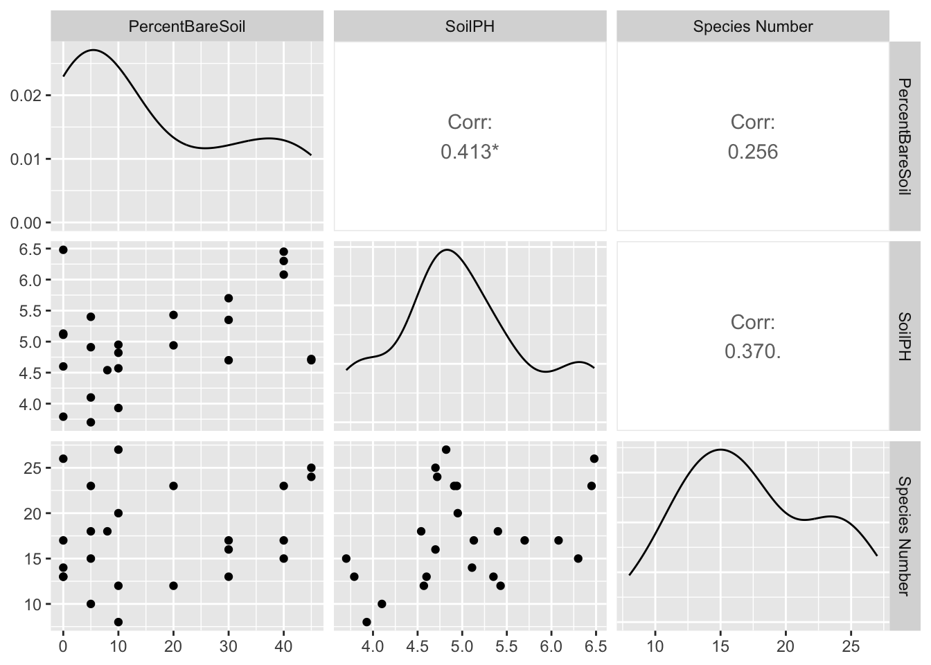
A weak correlation between soil pH and % bare soil, and a near-significant (0.05 < p < 0.1) correlation between soil pH and species number.
Note that if you only plan to use functions from a library a few times in your script it can be more efficient to call the function from the library once off using the syntax library::function (e.g.
GGally::ggpairs) than to attach the whole library (i.e. callinglibrary(GGally)) as it saves RAM.
That’s it! Go forth and conquer!