7 Going Bayesian

This section is also available as a slideshow. Right click or hold Ctrl or Command and click this link to view in full screen.

In this section I aim to provide a brief and (relatively) soft introduction to Bayesian statistical theory.

Iterative near-term ecological forecasting presents new challenges you don’t commonly encounter in the world of null hypothesis testing that has dominated ecology to date…

The iterative ecological forecasting cycle in the context of the scientific method, demonstrating how we stand to learn from making iterative forecasts.

While ecological forecasting and decision support can be done with traditional statistics (often termed “frequentist statistics”) it is generally much easier to do in a Bayesian statistical framework.

Bayesian approaches have several advantages for forecasting:

NOTE: there are frequentist approaches for doing much of this, but they are typically cumbersome “add-ons” that require many additional assumptions. Once you’re using Bayes you can achieve all this without much extra work.

1. They are typically focused on estimating what properties are (i.e. the actual value of a particular parameter) and not just establishing what they are not (i.e. testing for significant difference (null hypothesis testing), as is usually the focus in frequentist statistics)
2. They are highly flexible, allowing one to build relatively complex models with varied data sources (and/or of varying quality), especially Hierarchical Bayesian models
3. They can easily treat all terms as probability distributions, making it easier to quantify, propagate, partition and represent uncertainties throughout the analysis probabilistically. More on this later, but it addresses two of the key components of the ecological forecasting cycle:
   • being able to present the uncertainty in the forecast to the decision maker
   • being able to analyze the uncertainty in the forecast, in the hope that this can guide reducing the uncertainty and improving the next forecast, e.g. through targeted data collection or altering the model.
4. They provide an iterative probabilistic framework that mirrors the scientific method, allowing us to formalize learning from new evidence (i.e. new data) in the context of existing knowledge (prior information). This framework makes it easier to update predictions as new data become available, completing the forecasting cycle.

Before I can introduce Bayes, there are a few basic building blocks we need to establish first.

1. How the method of Least Squares works, and its limitations, especially it’s inflexible, implicit data model.
2. The concept of likelihood and the estimation of maximum likelihood, since this is a major component of Bayes’ Theorem. In fact, while likelihood is technically still a frequentist method, it has the advantages 1 & most of 2 above, without going full Bayes.

NOTE: This really is a minimalist introduction that only provides the tidbits I need you to know to follow the rest of the module. This note is a proviso to make it clear that I am withholding important details, before anyone accuses me of lies of ommission.

7.1 Least Squares

Traditional parametric statistics like regression analysis and analysis of variance (ANOVA) rely on Ordinary Least Squares (OLS). There are a few other flavours of least squares that allow a bit more flexibility (e.g. nonlinear (NLS) that we used in the practical in section ??, partial least squares, etc), but I’m not going to go into these distinctions.

In general, least squares approaches “fit” (i.e. estimate the parameters of) models by minimizing the sums of the squared residuals. Let’s explore this by looking at an example of a linear regression.

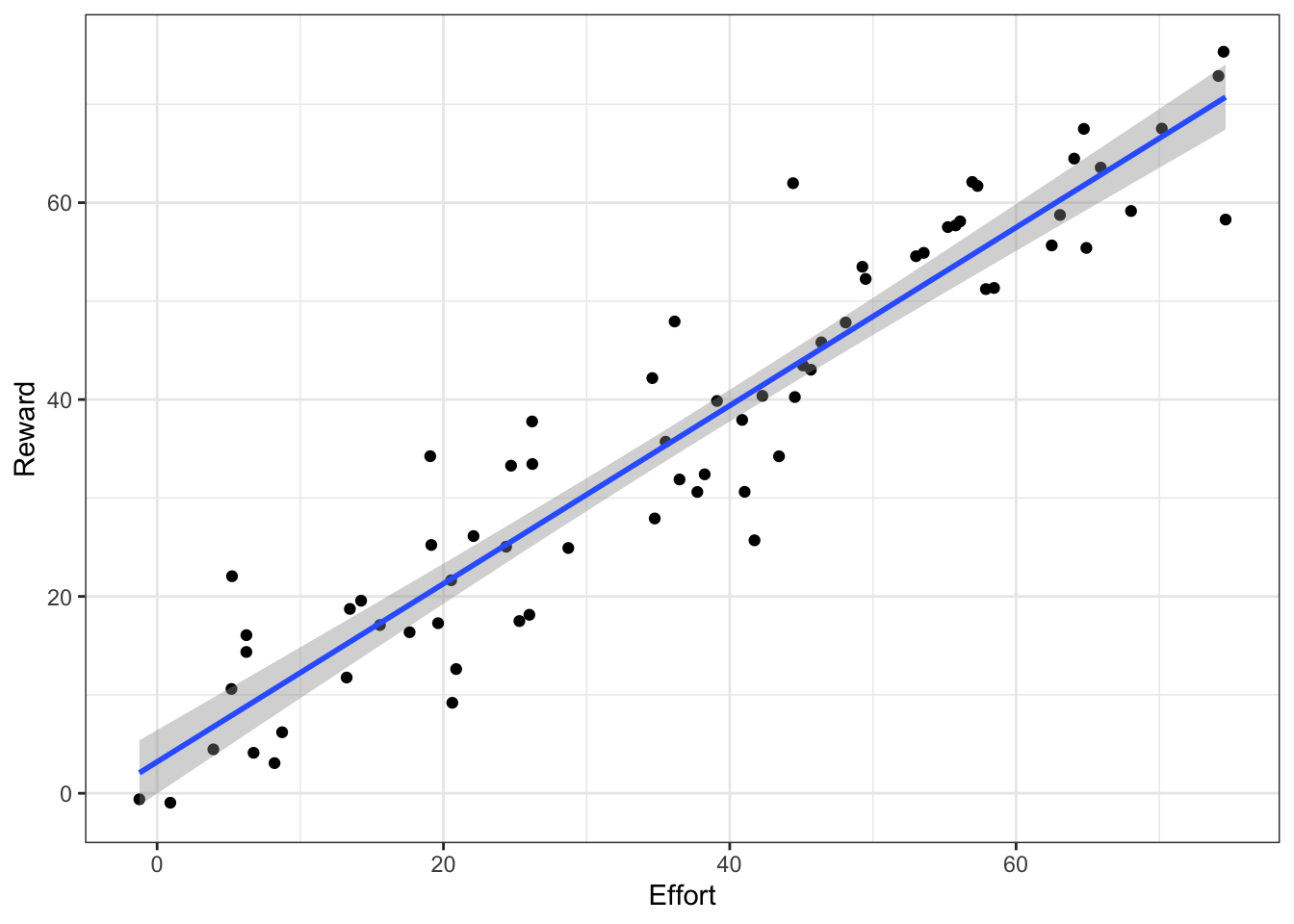
Figure 7.1: A hypothetical example showing a linear model fit.

Here the model (blue line) is drawn through the cloud of points so as to minimize the sum of the squared vertical (y-axis) differences (i.e. residuals) between each point and the regression line.

Let’s redraw this highlighting the residuals:

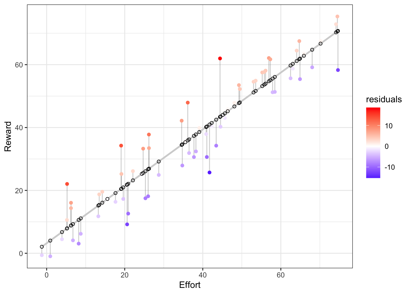
Figure 7.2: The linear model highlighting the residuals (lollypops) relative to the values predicted by the model (open circles along the regression line).

So the grey lines linking each observed data point to the regression line are the residuals. Note that they are vertical and not orthogonal to the regression line, because they represent the variance in Y (Reward in this case) that is not explained by X (Effort in this case). The open black circles are the Y-values that our linear model predicts for a given X-value. There is no scatter in the predicted values, because the scatter is residual variance that the model cannot account for and predict.

Now let’s have a look at a histogram of the residuals:

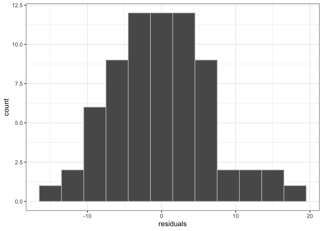
Figure 7.3: A histogram of the residuals from the linear model above.

In this case, the residuals approximate a normal distribution (or should, since I generated them from a normal distribution…). You’ll recall that this is one of the assumptions when using linear models or ANOVA (often termed “homoscedasticity” or “homogeneity of variance”) - i.e. it is an assumption of the Least Squares method. Least squares cannot handle residuals that are not normally distributed. If the residuals were not normally distributed, then either we are fitting the wrong model (e.g. we should consider a non-linear rather than a linear model), or our assumptions are violated and we should not be using this technique!

The reason Least Squares requires this assumption is that for minimizing the sums of squares to work, a unit change in the residuals should be scale invariant. In other words, the difference between 1 and 2 needs to be the same as the difference between 101 and 102. This is only the case when the residuals are normally distributed (versus log-scale for example). If the scale is variable, then minimizing the sums of squares does not work. People often try to get around the assumption of homogeneity of variance by tranforming their data (e.g. log or arcsine transform) to try to get them to an invariant scale.

So to look at the shortcomings of Least Squares:

7.1.1 Least Squares doesn’t explicitly include a data model

It’s useful at this stage to make a distinction between data models and process models.

• The process model is the bit you’ll be used to, where we describe how the model creates a prediction for a particular set of inputs or covariates (i.e. the linear model in the case above).
• The data model describes the residuals (i.e. the mismatch between the process model and the data). It is also often called the data observation process.

Least Squares analyses don’t explicitly include a data model, because the reliance on minimizing the sums of squares means that the data model in a Least Squares analysis can only ever be a normal distribution (i.e. homogeneity of variance).

This is a major limitation of the Least Squares method, because:

1. in reality, the data model can take many forms
   • e.g. Binomial coin flips, Poisson counts of individuals, Exponential waiting times, etc
   • this is where Maximum Likelihood comes into it’s own
     • recall that in the practical we specified two separate functions for the MLE analyses. One specified the process model (pred.negexp/S), the other specified the likelihood function (fit.negexp/S.MLE), which includes the data model.
2. there are times when one would like to include additional information in the data model
   • e.g. sampling variability (e.g. different observers or instruments), measurement errors, instrument calibration, proxy data, unequal variances, missing data, etc
   • this is where Bayesian models come into their own

7.1.2 Least squares focuses on what the parameters are not, rather than what they are

Least Squares focuses on significance testing - the ability to reject (or to fail to reject) the null hypothesis. In the case of a linear model, the null hypothesis is that the slope is zero (i.e. there is no effect of X on Y) and sometimes includes that the intercept should be zero too (although this is not usually required). I don’t have the time to go through the full explanation of how the null hypothesis is tested in this lecture, but it is useful to highlight that the linear model is only considered useful when you can reject the null hypothesis that the slope is zero (usually at an alpha of P < 0.05). While this is a start, it doesn’t tell you anything about the probability of the parameters actually being the estimates you arrives at by minimizing the sums of squares?!

7.2 Maximum likelihood

Maximum likelihood is a method used for estimating model parameters

The likelihood principle states a that parameter value is more likely than another if it is the one for which the data are more probable.

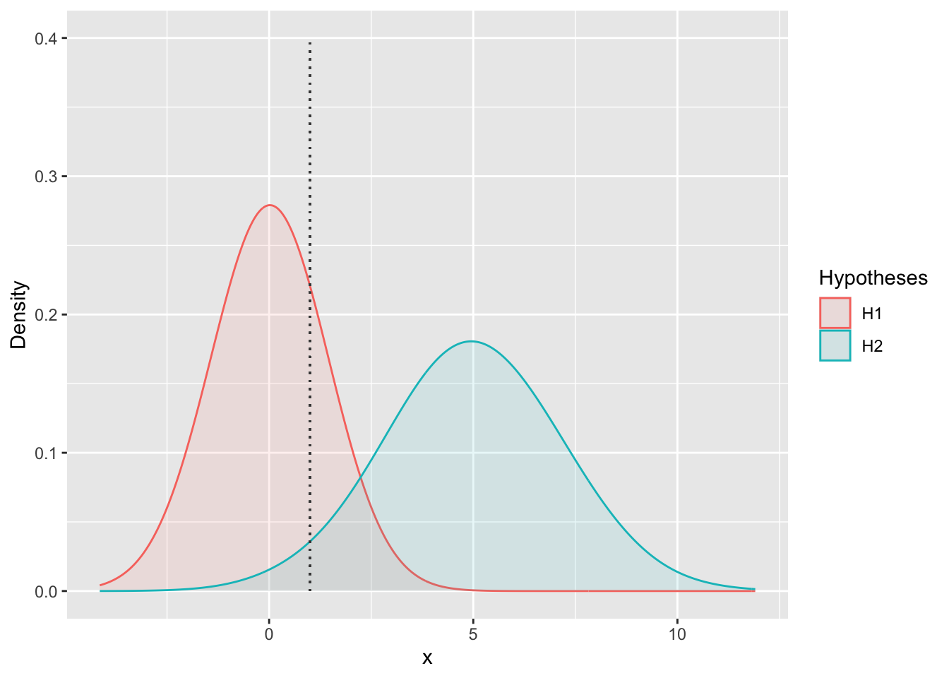
Figure 7.4: The probability of a observed point (the dotted line) being generated under two alternative hypotheses (sets of parameter values). In this case H1 is more likely, because the probability density at \(x\) = 1 is higher for H1 than H2 (roughly 0.25 vs 0.025). This makes H1 0.25/0.025 = 10 times more likely.

Maximum Likelihood Estimation (MLE) applies this principle by optimizing the parameter values such that they maximize the likelihood that the process described by the given model produced the data that were observed.

• To relate this to Figure 7.4, the parameter values would be a continuum of hypotheses to select from, and of course there would be far more data points that you’d need to calculate the probabilities for.

Viewed differently, when using MLE we assume that we have the correct model and apply MLE to choose the parameters so as to maximize the conditional probability of the data given those parameter estimates. The notation for this conditional probability is \(P(Data|Parameters)\).

This process leaves us knowing the likelihood of the best set of parameters and the conditional probability of the data given those parameters \(P(Data|Parameters)\).

The problem is that in the context of forecasting (and many other modelling approaches) what we really want is to know is the conditional probability of the parameters given the data \(P(Parameters|Data)\), because this allow us to express the uncertainty in the parameter estimates as probabilities³. To get there, we need to apply a little probability theory, which provides a somewhat surprising and very useful byproduct.

First, let’s brush up on our probability theory…

7.2.1 Joint, conditional and marginal probabilities

Here we’ll look at the interactions between two random variables and illustrate it with the Venn diagram below.

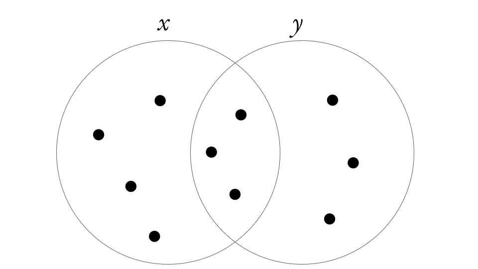
Figure 7.5: Venn diagram illustrating ten events (points) across two sets \(x\) and \(y\).

First, we can define the joint probability, \(P(x,y)\), which is the probability of both \(x\) and \(y\) occurring simultaneously, which in the case of Figure 7.5 is the probability of occurring within the overlap of the circles = 3/10. Needless to say the joint probability of \(P(y,x)\) is identical to \(P(x,y)\) (= 3/10).

Second, based on the joint probability we can define two conditional probabilities:

• the probability of \(x\) given \(y\), \(P(x|y)\), and
• the probability of \(y\) given \(x\), \(P(y|x)\).

In the context of the Venn diagram these would be:

• the probability of being in set \(x\) given that we are only considering the points in set \(y\) (= 3/6), and
• the probability of being in set \(y\) given that we are only considering the points in set \(x\) (= 3/7).

Last, we can define two marginal probabilities for \(x\) and \(y\), which are just the separate probabilities of being in set \(x\) or being in set \(y\) given the full set of events, i.e.:

• \(P(x)\) = 7/10 and
• \(P(y)\) = 6/10.

We can also show that the joint probabilities are the product of the conditional and marginal probabilities:

\[\begin{align*} P(x,y) = P(x|y) P(y) = 3/6 * 6/10 = 0.3 \end{align*}\]

And by the same token:

\[\begin{align*} P(y,x) = P(y|x) P(y) = 3/7 * 7/10 = 0.3 \end{align*}\]

Why I’m telling you all this is because knowing this last equation (that the joint probabilities are the product of the conditional and marginal probabilities) means that we can derive the information we want to know, \(P(Parameters|Data)\), as a function of the information maximum likelihood estimation has given us, \(P(Data|Parameters)\)…

7.3 Bayes’ Theorem

From here I’ll refer to the parameters as \(\theta\) and the data as (\(D\)), because writing them out in full is a bit clunky and grownups don’t usually do that.

Since we are interested in the conditional probability of the parameters given the data, \(p(\theta|D)\), we need to take the equations above and solve for \(p(\theta|D)\).

From above, we know

\[\begin{align*} p(\theta,D) = p(\theta|D)p(D) \end{align*}\]

and we know that the joint probabilities are identical, so we can also write

\[\begin{align*} p(\theta,D) = p(D|\theta)p(\theta) \end{align*}\]

so we can rewrite this to compare the right hand side of the last two equations

\[\begin{align*} p(\theta|D)p(D) = p(D|\theta)p(\theta) \end{align*}\]

which if we solve for \(p(\theta|D)\) is

\[\begin{align*} p(\theta|D) & = \frac{p(D|\theta) \; p(\theta)}{p(D)} \;\; \end{align*}\]

which is known as Bayes’ Theorem.

7.3.1 The beauty of Bayes’ Theorem

Now let’s unwrap our birthday present and see what we got!

Rewriting the terms on one line allows us to label them with the names by which they are commonly known:

\[ \underbrace{p(\theta|D)}_\text{posterior} \; = \; \underbrace{p(D|\theta)}_\text{likelihood} \;\; \underbrace{p(\theta)}_\text{prior} \; / \; \underbrace{p(D)}_\text{evidence} \] First, let’s start with the last term, the evidence as this will allow us to simplify things.

The marginal probability of the data, \(p(D)\), is now called the evidence for the model, and represents the overall probability of the data according to the model, determined by averaging across all possible parameter values weighted by the strength of belief in those parameter values.

This sounds quite complicated, but never fear, all you need to know is that the implication of having \(p(D)\) in the denominator is that it normalizes the numerators to ensure that the updated probabilities sum to 1 over all possible parameter values. In other words, the evidence term ensures that the posterior, \(p(\theta|D)\), is expressed as a probability distribution, and can otherwise mostly be ignored.

This allows us to focus on the important bits, and to express Bayes’ Rule as

\[ \underbrace{p(\theta|D)}_\text{posterior} \; \propto \; \underbrace{p(D|\theta)}_\text{likelihood} \;\; \underbrace{p(\theta)}_\text{prior} \; \]

Which reads “The posterior is proportional to the likelihood times the prior”.

This leaves us with three terms.

First, we have the likelihood, \(p(D|\theta)\). This is unchanged and still represents the probability that the data could be generated by the model with parameter values \(\theta\), and when used in analyses still works to find the likelihood profiles of the parameters.

Next, what we have been calling the conditional probability of the parameters given the data, \(p(\theta|D)\), is now called the posterior, and represents the credibility of the parameter values \(\theta\), taking the data, \(D\), into account. In other words, it gives us a probability distribution for the values any parameter can take, essentially allowing us to represent uncertainty in the model and forecasts as probabilities, which is the holy grail we were after!!!

Last, we’ll look at the marginal probability of the parameters, \(p(\theta)\), which is now called the prior. While \(p(\theta)\) is almost an unexpected consequence of having solved the equation for \(p(\theta|D)\), this is where the magic lies! Firstly, we know that \(p(\theta)\) is a necessary requirement for us to be able to represent the posterior, \(p(\theta|D)\), as a probability distribution. That it helps us do this is magic in itself, but what is \(p(\theta)\) itself?

The prior represents the credibility of the parameter values, \(\theta\), without the data, \(D\).

How can we know anything about the parameter values without the data you may ask? In short, the answer is because we are applying the scientific method, whereby we interrogate new evidence (the data) in the context of previous knowledge or information to update our understanding. The term \(p(\theta)\) is called the prior, because it represents our prior belief of what the parameters should be, before interrogating the data. In other words, the prior is our “context of previous knowledge or information”. The nice thing is that if we don’t have much previous knowledge or information, we can specify the prior to represent that.

The prior is incredibly powerful, but, as always the Peter Parker Principle applies - “With great power comes great responsibility!”

The prior is incredibly powerful, because:

1. It allows Bayesian analyses to be iterative. The posterior from one analysis can become the prior for the next!
   • This provides a formal probabilistic framework for the scientific method! New evidence must be considered in the context of previous knowledge or information, and provides us the opportunity to update our beliefs.
   • This is also ideal for iterative forecasting, because the previous forecast can be the prior for the next, (and the observed outcome of the previous forecast window can be the new data that’s fed into the likelihood function for the next forecast).
2. It makes Bayesian modelling incredibly flexible by allowing us to specify complex models like hierarchical models in a completely probabilistic framework relatively intuitively.
   • For example, in some cases we may not have any strong direct “prior beliefs” about the parameter values, but we may know something about another parameter or process that influences the parameter value of interest. In this case we can specify a prior on our prior (usually called a hyperprior).
   • Another key component here is that we can specify separate or linked priors or hyperpriors for different parameters or priors.

The prior also comes with great responsibility, because:

In short, it is very easy to specify an inappropriate prior and bias the outcome of your analysis!

• First and foremost, as tempting as it may be, the one place the prior CANNOT come from is the data used in the analysis!!!
• Second, while many people favour specifying “uninformative” priors, it is often incredibly difficult to know what “uninformative” is for different models or parameters.
  • For example, say you were trying to build a model to solve a murder mystery and predict who the likely culprit is. One of the parameters may be the gender of the culprit. If you’re lazy, you may say “we set an uninformative prior that there was a 50/50 chance of the culprit being male or female”. In truth, this “uninformative” prior may well bias your result for a number of reasons:
    • Firstly, sex ratios are rarely 50/50 (e.g. in South Africa a quick Google search suggests the M/F ratio is supposedly 1:1.03). In this case your prior would be unfairly biasing the model towards predicting that that the culprit is a woman.
    • Acknowledging this, you may then set your sex ratio as the observed ratio for the population in the region where the murder took place, but there are further complexities that may bias your results. e.g. Observed data suggest that far more men commit murder than women, but going with the observed sex ratio for the population makes the assumption that men and women are equally likely to commit murder.
    • Next, your prior has not taken into account the profile of the victim - man, woman, child, etc - but the sex ratios of murderers varies hugely whether you’re considering androcide, femicide or infanticide.
    • Lastly, what about gender identity and sexual orientation (LGBTQI+)? Have your sources of prior information taken this into account and would this affect the outcome?

Here’s a great Guardian article on why considering priors are important for Covid testing and criminal cases. It should help you get your head around this.

We’ll get stuck into examples showing the value of Bayes in ecological studies in the next lecture.

---

3. Note that we have the likelihood of the parameter estimates, but \(likelihood \neq probability\). I don’t want to spend time on the distinction in the lecture, but it is a very important concept. The area under a probability distribution sums to 1, but the area under a likelihood profile curve does not. The reason for this is that probability relate to the set of possible results, which are exhaustive and mutually exclusive, whereas likelihood relates to the possible hypotheses, which are neither exhaustive nor mutually exclusive (i.e. there’s no limit to the number of potential hypotheses, and hypotheses can be nested or overlapping).↩︎