11 Completing the forecast cycle

Here we’ll complete the forecast cycle (through data assimilation) and spend a little time discussing decision support.

11.1 Data assimilation

Figure 11.1: The iterative ecological forecasting cycle in the context of the scientific method, demonstrating how we stand to learn from making iterative forecasts. From lecture on data assimilation by Michael Dietze. (Please excuse that the colours of the distributions have changed from above…).

You’ll recall from the introductory lecture on models and decision making (section 3) that we outlined iterative ecological forecasting and the scientific method as closely aligned cycles or loops. You’ll also recall that I made the point in section 7 that Bayes Theorem provides an iterative probabilistic framework that makes it easier to update predictions as new data become available, mirroring the scientific method and completing the forecasting cycle. Here we’ll unpack this in a bit more detail.

11.1.1 Operational data assimilation

Most modelling workflows are set up to (a) fit the available data and estimate parameters etc (we’ll call this analysis), which they then often use to (b) make predictions (which if made forward through time are typically forecasts). They usually stop there. Few workflows are set up to make forecasts repeatedly or iteratively, updating predictions as new observations are made.

When making iterative forecasts, one could just refit the model and entire dataset with the new observations added, but there are a few reasons why this may not be ideal:

1. If it’s a complex model and/or a large dataset this could be very computationally taxing -e.g. Slingsby, Moncrieff, and Wilson (2020) ran the Hierarchical postfire model for the Cape Peninsula (~4000 MODIS pixels) over 4 days on a computing cluster with 64 cores and 1TB of RAM…
2. Depending on the model, you may not be able to reuse older data in the new model fit, meaning you can’t take advantage of all available data…
3. Refitting the model doesn’t make the most of learning from new observations and the forecast cycle…

The alternative is to assimilate the data sequentially, through forecast cycles, imputing observations a bit at a time as they’re observed. This approach has several advantages:

1. They can handle larger datasets, because you don’t have to assimilate all data in one go.
2. If you start the model far in the past and update towards present day, you have the opportunity to validate your predictions, telling you how well the model does, and whether it improves with each iteration (i.e. is it learning), which gives you a good feel for how well it should do at forecasting into the future. Think of it as letting your model get a run-up like a sportsperson before jumping/bowling/throwing.

Assimilating data sequentially is known as the sequential or operational data assimilation problem and occurs through two steps (the main components of the forecast cycle), the forecast step, where we project our estimates of the current state forward in time, and the analysis step, where we update our estimate of the state based on new observations.

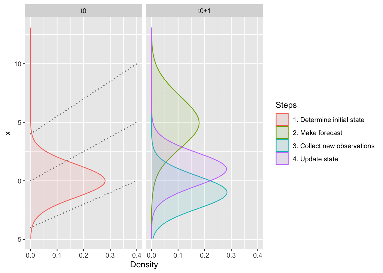
Figure 11.2: The two main components of the forecast cycle are the forecast step (stippled lines), where we project from the initial state at time 0 (\(t_0\)) to the next time step (\(t_{0+1}\)), and the analysis step, where we use the forecast and new observations to get an updated estimate of the current state at \(t_{0+1}\), which would be used for the next forecast to \(t_{0+2}\).

11.1.2 The Forecast Step

While it gets a bit like the chicken and the egg dilemma, the first step has to be analysis, because you have to fit your model before you can make your first forecast (although you could argue that your first analysis requires priors, which could be viewed as your first forecast…).

Either way, the forecast step is probably easier to explain first.

The goals of the forecast step are to:

1. To predict what we think may happen (or what the state variable(s) will be) at the next time step
2. Indicate the uncertainty in our forecast (based on the uncertainty that we have propagated through our model from various sources (data, priors, etc))

In short, we want to propagate uncertainty in our variable(s) of interest forward through time (and sometimes through space, depending on the goals).

There are a number of methods for propagating uncertainty into a forecast, mostly based on the same methods one would use to propagate the uncertainty through a model (see Table 10.1). Explaining the different methods more than I did in section (10) is beyond the scope of this module, but just a reminder that (as with almost everything in statistics) there’s a trade-off between the methods whereby the most efficient (the Kalman filter in this case) also come with the most stringent assumptions (linear models and homogeneity of variance only), while the most flexible (Markov chain Monte Carlo (MCMC) in this case - a Bayesian approach) are the most computationally taxing. In short, if your model isn’t too taxing, or you have cheap access to a very large computer and time to kill, MCMC is probably best (and often easiest if you’re already working in Bayes)…

11.1.3 The Analysis Step

NOTE: I’m only explaing the general principles for doing this in a Bayesian framework. There are approaches listed in Table 10.1 that can be implemented in a frequentist framework, but (lucky for you) I’m not going to go there.

This step involves using Bayes Theorem to combine our prior knowledge (our forecast) with our new observations (at \(t_{0+1}\) in Figure 11.2) to generate an updated state for the next forecast (i.e. to \(t_{0+2}\)).

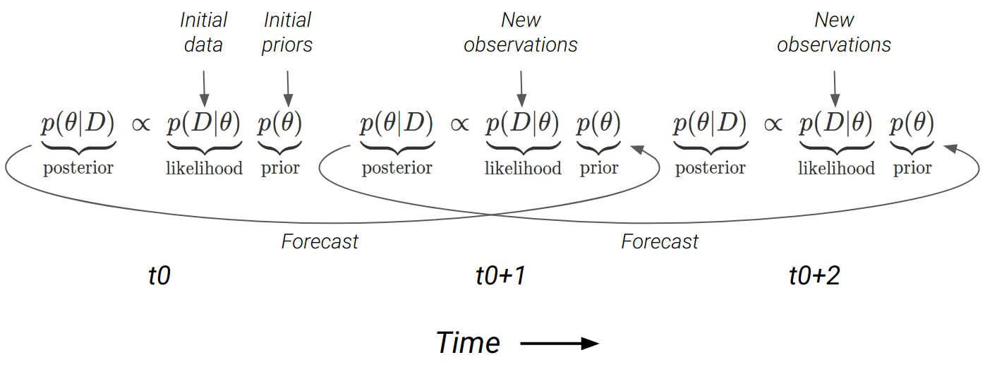
Figure 11.3: The forecast cycle chaining together applications of Bayes Theorem at each timestep (\(t_0, t_1, ...\)). The forecast from one timestep becomes the prior for the next. Note that the forecast is directly sampled as a posterior distribution when using MCMC, but can also be propagated using other methods (see Table 10.1).

This is better than just using the new data as your updated state, because:

• it uses our prior information and understanding
• it allows our model to learn and (hopefully) improve with each iteration
• there is likely error (noise) in the new data, so it can’t necessarily be trusted more than our prior understanding anyway

Fortunately, Bayes Theorem deals with all of this very nicely, because if the forecast (prior) is uncertain and the new data precise then the data will prevail, whereas if the forecast is precise and the new data uncertain, then the posterior will retain the legacy of previous observations (Figure 11.4).

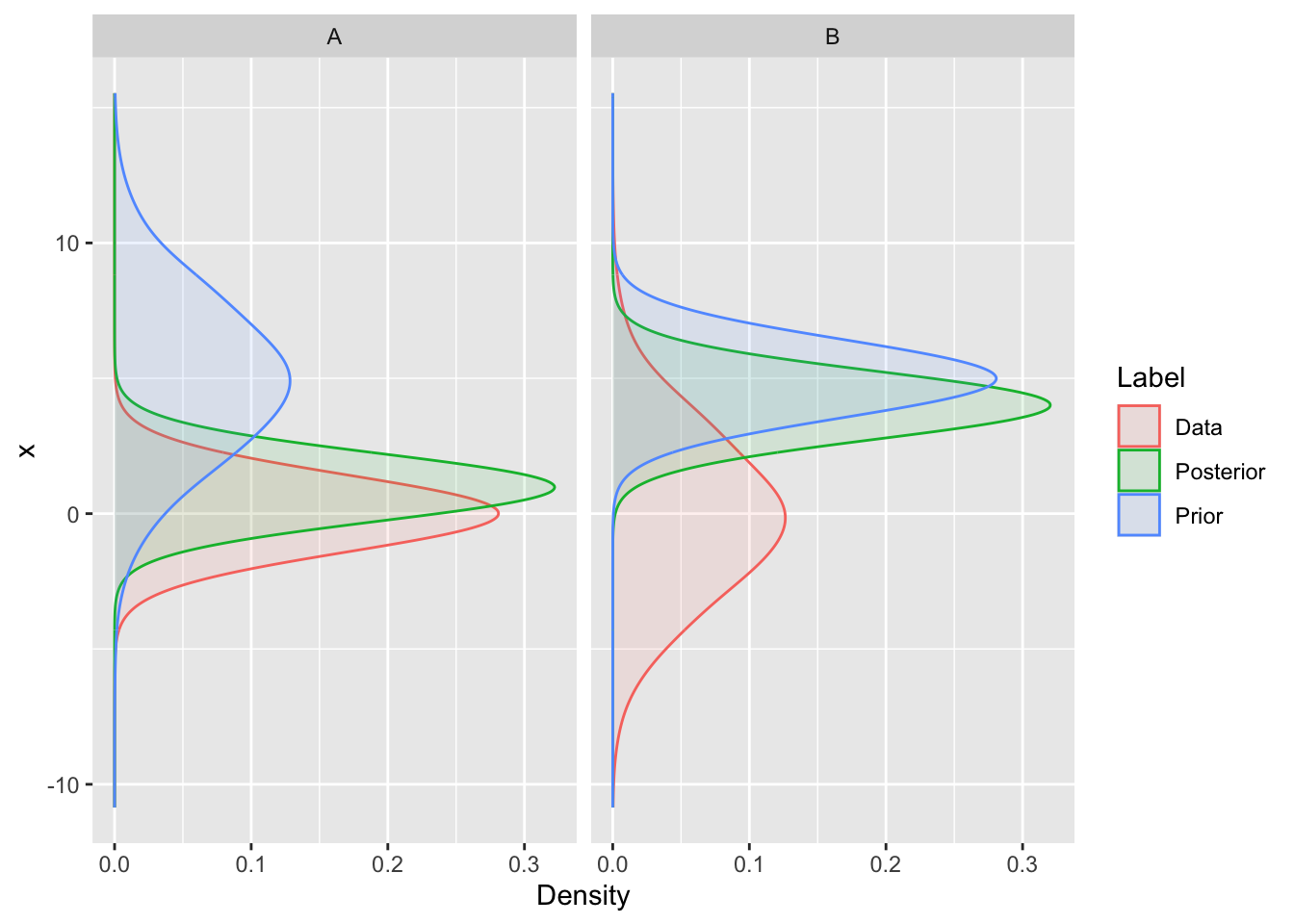
Figure 11.4: The result of (A) high forecast uncertainty (the prior) and low observation error (data), and (B) low forecast uncertainty and high observation error on the posterior probability from the analysis step. Note that the data and prior have the same means in panels A and B, but the variances differ.

Lastly, just a note that I’ve mostly dealt with single forecasts and haven’t talked about how to deal with ensemble forecasts. In short, there are data assimilation methods to deal with them, but we don’t have time to cover them. The methods, and how you apply them, depend on what kind of ensemble you are dealing with. Usually, ensembles can be divided into three kinds, but you can have mixes of all three:

1. Where you use the same model, but vary the inputs to explore different scenarios.
2. Where you have a set of nested models of increasing complexity (e.g. like our postfire models with and without the seasonality term).
3. A mix of models with completely different model structures aimed at forecasting the same thing.

11.2 Decision support

This is probably the hardest part of the whole ecological forecasting business… people!

It is also a huge topic and not one I can cover in half a lecture. Here I just touch on a few hints and difficulties.

First and foremost, the decision at hand may not be amenable to a quantitative approach.

• Ecological forecasting requires a clearly defined information need with a measurable (and modelable) state variable, framed within one or multiple decision alternatives (scenarios).
• There’s also the risk of external factors making the forecasts unreliable, especially if they are not controlled by the decision maker and/or their probability is unknown (e.g. fire, pandemics, etc).

These external factors are where developing scenarios with different boundary conditions can be very useful

• e.g. a scenarios with and without a fire, or the different future climate states under the alternative development pathways, etc.
• Scenarios are often “what if” statements designed to address major sources of uncertainty that make it near-impossible to make accurate predictions with a single forecast.

It’s perhaps useful to note the distinction between predictions versus projections at this point:

• predictions are statements about the probability of the occurrence of events or the state of variables in the future based on what we currently know
• projections are statements about the probability of the occurrence of events or the state of variables in the future given specific scenarios with clear boundary conditions

If the prerequisites to be able to do ecological forecasting are met, then…

11.2.1 In an ideal world…

You’ll be working with an organized team that is a well-oiled machine at implementing Adaptive Management and Structured Decision Making and you can naturally slot into their workflow.

The advantages of Adaptive Management and Structured Decision Making are that they are founded on the concept of iterative learning cycles, which they have in common with the ecological forecasting cycle and the scientific method.

Figure 11.5: Conceptual relationships between iterative ecological forecasting, adaptive decision-making, adaptive monitoring, and the scientific method cycles (Dietze et al. 2018).

You’re already familiar with how the iterative ecological forecast cycle integrates with the Adaptive Management Cycle…

The beauty for the forecaster in this scenario is that a lot of the work is already done.

• The decision alternatives (scenarios) have been well framed.
• The performance measures, state variables of interest and associated covariates mostly identified.
• Iterations of the learning cycle may even have already begun (through the Adaptive Management Cycle) and all you need do is develop the existing qualitative model into something more quantitative as more data and understanding are accumulated.
  • Think of the Protea example in section 4, where the demography of these species is already used for decision making using semi-quantitative “rules of thumb”.

Structured Decision Making

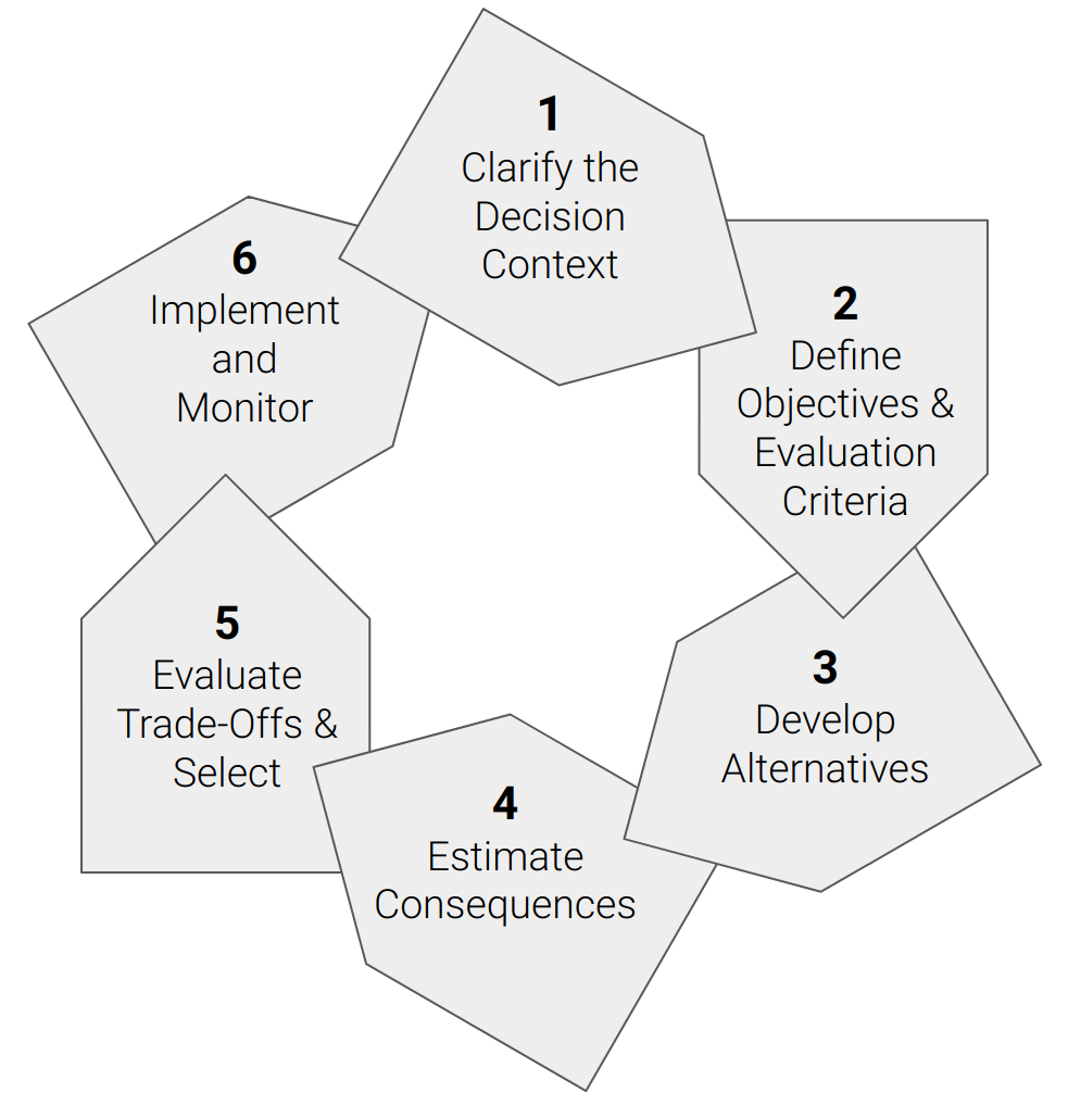
Figure 11.6: The Structured Decision Making Cycle sensu Gregory et al. (2012).

As the name suggests, Structured Decision Making is far more focused on assisting with the process of coming to a decision than the process of management, but it is particularly useful in the first iteration of the Adaptive Management Cycle. Gregory et al. (2012) provide a very nice magnum opus on Structured Decision Making in natural resource management. It is particularly valuable when there are many stakeholders with disparate interests.

We can model properties and performance measures, but decisions are ultimately about values and often require evaluating trade-offs among properties with incomparable units, e.g. people housed/fed/watered vs species saved from extinction… This can rapidly become a highly emotive space. It is also a space where the values that dominate are often the ones that are shouted the loudest and other important values are marginalized.

• One of the major goals of Structured Decision Making is to make sure all issues and values are brought to light and considered in a transparent framework so that trade-offs can be clearly identified and considered.
• It also aims to ensure that all alternatives are considered, since it’s impossible to make the right choice if it isn’t even on the table.

A key strength in Structured Decision Making is in attempting to directly address the social, political or cognitive biases that limit the ability to highlight all values or alternatives.

• e.g. many decisions in South Africa (and globally) pit people’s immediate needs (water, housing, etc) against the environment. These are incredibly difficult decisions, and while people (especially politicians) would rather ignore the fact that choosing one is choosing against the other, if we’re not transparent about this we’re not going to learn from our decisions and improve them in the next iteration.

11.2.2 In reality…

Many (if not most) decisions are made with very little information and/or within institutional structures that are not well designed for iterative learning and adaptation.

In fact, you’ll often encounter situations where people aren’t interested in the information you have to offer, even if it’s exactly what they need. You may often find they don’t know what they need, so you may need to tell them, if you can get the chance… This may well be met with resistance, because you’re adding what is perceived to be unnecessary complexity to an otherwise straightforward decision scenario (e.g. many engineers prefer to ignore environmental concerns - the first step is often just making sure that the environment is even considered among the objectives and performance measures…).

That said, you should also have the humility recognize that it is very possible that what you have to offer is not what the decision maker needs, despite your own preconceptions.

Effective engagement with decision makers requires a lot of empathy (putting yourself in their shoes) and willingness to listen, combined with a good dose of taking them to task when needed (i.e. when they’re ignoring important information out if ignorance or conveniance). You’re unlikely to know the full complexity and constraints of the institutional (and legal) frameworks within which they have to work. They may well be on your side personally, but can’t show that formally. That said, they may be overly blinkered by their institutional frameworks and norms and need a little disruption to force them to think outside the box.

There’s also a tricky balance between knowing what you can offer (based on the available data and the various factors that determine whether you can develop a useful forecast) and learning what is needed (either from or by working with decision makers). On the one hand, designing an “over-the-wall” forecasting solution without engagement with stakeholders is unlikely to be well received. On the other hand, discussion of potential forecasting solutions with decision makers does need to be constrained by the reality of the limits to forecasting, otherwise you may be asked to (or worse - you may promise to) deliver on an impossible forecasting task. “Unconstrained” discussions typically lead to time-wasting and anymosity - “Why were we discussing this if it was never a possibility?!”

In many ways working with decision makers is about slowly building relationships and exploring possibilities together, possibly focusing on one or a few allies who see the potential value early. If you can use their input to help develop something useful, it becomes much easier to demonstrate realistic value to the broader group, often championed by your allies. Then you’re well placed to refine and improve it.

11.3 Final words

We need to move past the traditional ecologist’s view:

After decades’ worth of data collection and hypothesis testing, maybe we’ll know enough to start building a predictive model…

And start adopting an engineering (or decision-makers’) view (at least one that subscribes to some iterative learning paradigm):

Start building a model with what we have, even if there is little or no data, and use that to guide what data to collect and how to improve the model. It may be completely wrong to begin with, but will rapidly improve.

11.4 Revision questions

Because you asked so nicely…

These would all be essay questions (30-50 marks, with how much you write depending on the mark and time allocation).

• Discuss the main requirements for data used in ecological forecasts and how they may (or may not) be resolved through adherence to the Data Life Cycle.

• Why is there a crisis in the way we do science, what can we do about it, and what are the additional benefits?

• Write a convincing motivation why staff and students should be conducting their research reproducibly, and explain some of the requirements for achieving this.

• What are the benefits of Bayesian approaches over other statistical frameworks in the context of ecological forecasting and how does the Bayesian framework make them possible?

• Discuss the ways in which one can fuse data with models and how this may be limited by your statistical approach.

• You have been tasked with improving the proficiency of an ecological forecasting model. Discuss the potential sources of uncertainty, how you would identify them and deploy limited resources to reduce them.

• Discuss the ecological forecasting cycle and how it integrates with and accelerates learning within existing management and knowledge generation frameworks.

References

Dietze, Michael C, Andrew Fox, Lindsay M Beck-Johnson, Julio L Betancourt, Mevin B Hooten, Catherine S Jarnevich, Timothy H Keitt, et al. 2018. “Iterative near-term ecological forecasting: Needs, opportunities, and challenges.” Proceedings of the National Academy of Sciences of the United States of America 115 (7): 1424–32. https://doi.org/10.1073/pnas.1710231115.

Gregory, Robin, Lee Failing, Michael Harstone, Graham Long, Tim McDaniels, and Dan Ohlson. 2012. Structured Decision Making: A Practical Guide to Environmental Management Choices. John Wiley & Sons.

Slingsby, Jasper A, Glenn R Moncrieff, and Adam M Wilson. 2020. “Near-real time forecasting and change detection for an open ecosystem with complex natural dynamics.” ISPRS Journal of Photogrammetry and Remote Sensing: Official Publication of the International Society for Photogrammetry and Remote Sensing 166 (August): 15–25. https://doi.org/10.1016/j.isprsjprs.2020.05.017.