5 Some important concepts and pitfalls

5.1 Scale

All maps have a scale. Scale is the ratio between the size of the representation of an object and its size in reality. E.g. objects on a 1:50,000 scale map are drawn at 1/50,000 their size, so 1cm on the map represents a distance of 500m in reality (i.e. \(1*50,000 = 50,000cm = 500m\)).

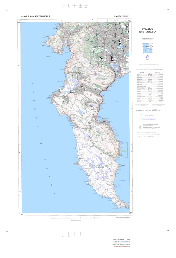
Figure 5.1: The Cape Peninsula (3418AB & AD) from South Africa’s 1:50,000 topographic map series. The printed scale for these maps is 1:50,000, but what is it on your screen?

GIS is usually scaleless (or at least flexible in scale); we can “zoom in” as much as we want to, and perform operations at just about any scale we want to, but should we? There are lots of issues we need to consider!

• Representation (i.e. mapping)… There are 2 issues here:
  • Firstly, a 1mm thick line on a 1:50,000 scale map would be 50m wide in reality. Conversely, a 5m wide road would be 1/10mm on the map. Would the map be readable? Sometimes we break the rules of scale to make maps readable. Bear this in mind!
  • Secondly, scale and our desired representation affect how we capture data. For example, a road is typically best represented as a line at 1:5,000 scale or smaller (note that scale is a ratio, so “small scale” = large extent or area!). At 1:1,000 scale a 5m wide road would be 5mm across on the map, so one might capture it as a polygon to represent its area. You should always consider the purpose for which (and scale at which) the data were captured before using them for a new application! This affects both the appropriateness of the data type and the accuracy and precision of the data…

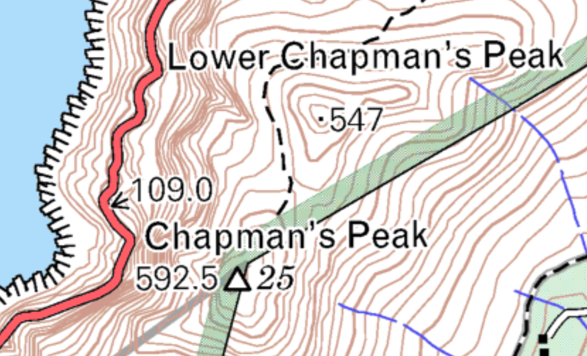
Figure 5.2: Zoomed in on Chapman’s peak on the the Cape Peninsula 1:50,000 topographic map (3418AB & AD). At this scale the road (in red) is probably better mapped as an area than a line?

• Accuracy of location versus scale of data capture. We should always check the scale at which the data were captured to make sure it is accurate enough for the scale of the analysis we are doing. For example, the various vegetation units in the National Vegetation Map of South Africa were mapped at a range of scales, some as small as 1:250,000. At this scale 1mm = 250m, so a minor digitization error is a huge difference on the ground! If you need your analysis to be accurate to <10m then you’d probably need data mapped at a scale larger than 1:10,000.
• Precision - Can mean two things:
  • The unit or number of decimal places to which the attribute has been measured (and can be stored)
  • The spread of repeat measurements (typically in field data collection). A big spread means the measurements weren’t very precise…

A quick aside on the difference between accuracy and precision!

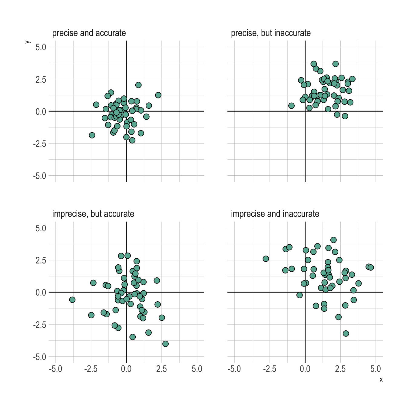
Figure 5.3: The difference between accuracy and precision, where the true value is the origin (0,0).

A last word on Scale…

For vector data, we typically refer to scale when describing a data set.

For raster data, we typically refer to pixel resolution (or sample interval). For example, a 30m digital elevation model is made up of pixels 30m across. For remotely sensed imagery (i.e. from drone, plane or satellite), one often uses the term “ground sample distance”.

BEWARE!!! If you convert between raster and vector data formats (e.g. by “rasterizing” a vector layer, or “binning” a raster into polygons), it will affect all three of precision, accuracy and representation, so you need to give careful thought to whether what you are doing is appropriate for the analysis you are doing!

5.2 Coordinate Reference Systems (CRS)

Coordinate Reference Systems (CRS) provide a framework for defining real-world locations. There are many different CRSs, with different properties. They can be a minefield, and I don’t have the time to cover them in any detail. I provide some of the basics here, and list some of the golden rules (mostly from the GIS Support Unit) below.

5.2.1 Geographic (or “unprojected”) Coordinate Systems

The most common coordinate system is latitude/longitude, also known as geographic, lat/long or sometimes WGS84. There are many ways to record geographic coordinates:

• Degrees, Minutes & Seconds: S33°26’46”,E18°10’23’’
• Degrees and decimal minutes: S33°26.7666667’,E18°10.3833333’ (out to get you!)
• Decimal Degrees: -33.4461111,18.17305556

Most GIS prefer decimal degrees…

The problem with doing analyses using geographic CRS is that lat/long coordinates are actually angular measurements on a 3D sphere (Geodesic) and degrees differ in their actual ground distance depending on where you are on the planet. They also differ in the N-S vs W-E plane!

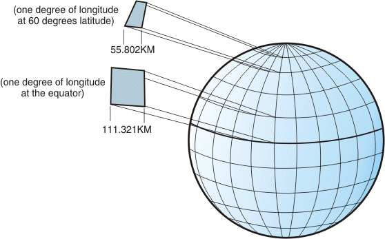
Figure 5.4: Map highlighting that a degree is larger at the equator than at the poles. Image source: https://annakrystalli.me/intro-r-gis/gis.html

This means that Euclidean measurement calculations are not appropriate for calculating areas and distances on data in the geographic CRS.

5.2.2 Projected Coordinate Systems

To perform linear measurements from a 3D shape using Euclidean methods, you need to squash that shape into a 2D plane. This squashing is called a projection…

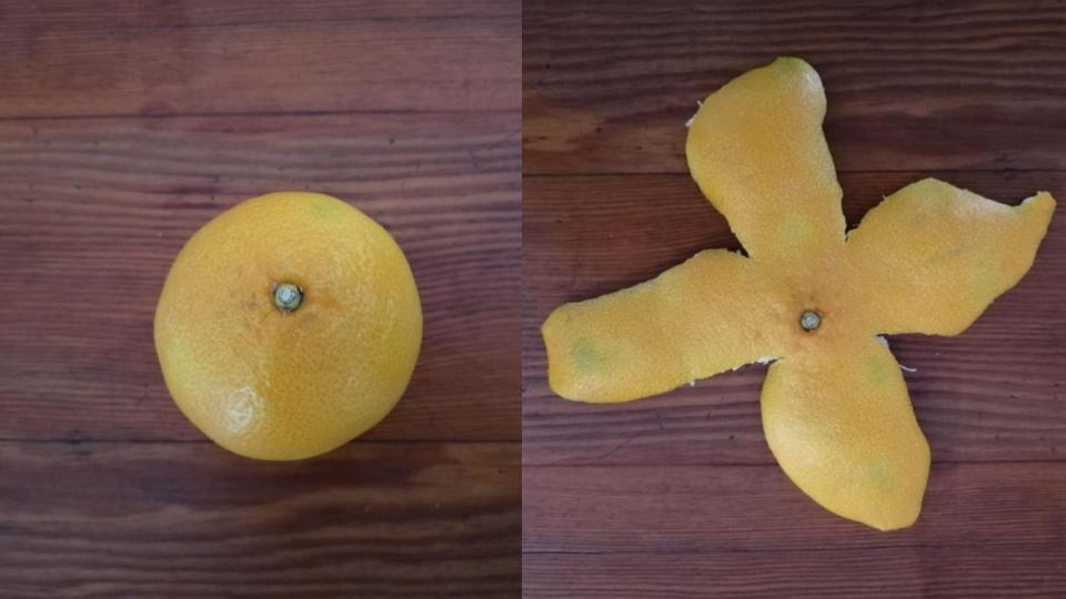
Figure 5.5: How many different ways could you flatten a naartjie peel?

There are 4 properties that get distorted, you can pick which one gets preserved the best by a projection type:

• Shape - you want a Conformal projection
• Area - Equal-Area
• Distance - Equidistant
• Direction - Azimuthal

(see here for a nice description and illustrations)

Some “general purpose” projections, like Transverse Mercator (TM), try to compromise and minimize distortion in all properties, but can’t preserve any perfectly. Their distortions also tend to get worse the larger the spatial extent being analyzed.

Projections get tuned to best fit an area through the use of projection parameters. For example, Transverse Mercator, which is used by the 1:50,000 map series and by Municipalities like Cape Town, uses a narrow projection window of 2 degree-wide bands. As a result, our map series projection parameters are set by moving the central meridian (or tangent) line of longitude every odd degree across the country. Cape Town is close to 19°E, so our version is colloquially called ‘Lo19’. For Durban you’d use ‘Lo31’. Universal Transverse Mercator (UTM) is similar, but uses 6 degree-wide bands so that it can be applied across larger extents.

5.2.3 Projection codes

The type of CRS is usually (but not always) stored in the metadata of your file (or dataset, if it is comprised of multiple files like an ESRI shapefile). There are various formats for this, the most commonly used in R being known as EPSG, PROJ4 or WKT codes or strings (be warned, there are many more…).

To assign a CRS or reproject your data in R you need to know the appropriate code in the format required by the function. Fortunately, there is a huge online library of the codes at https://spatialreference.org/. I also provide some suggested projections, based on the properties you’d like to preserve, and their codes here. Note that for UTM and TM you may need to adjust the PROJ4 strings for your area - read the comments.

Why do projections matter?

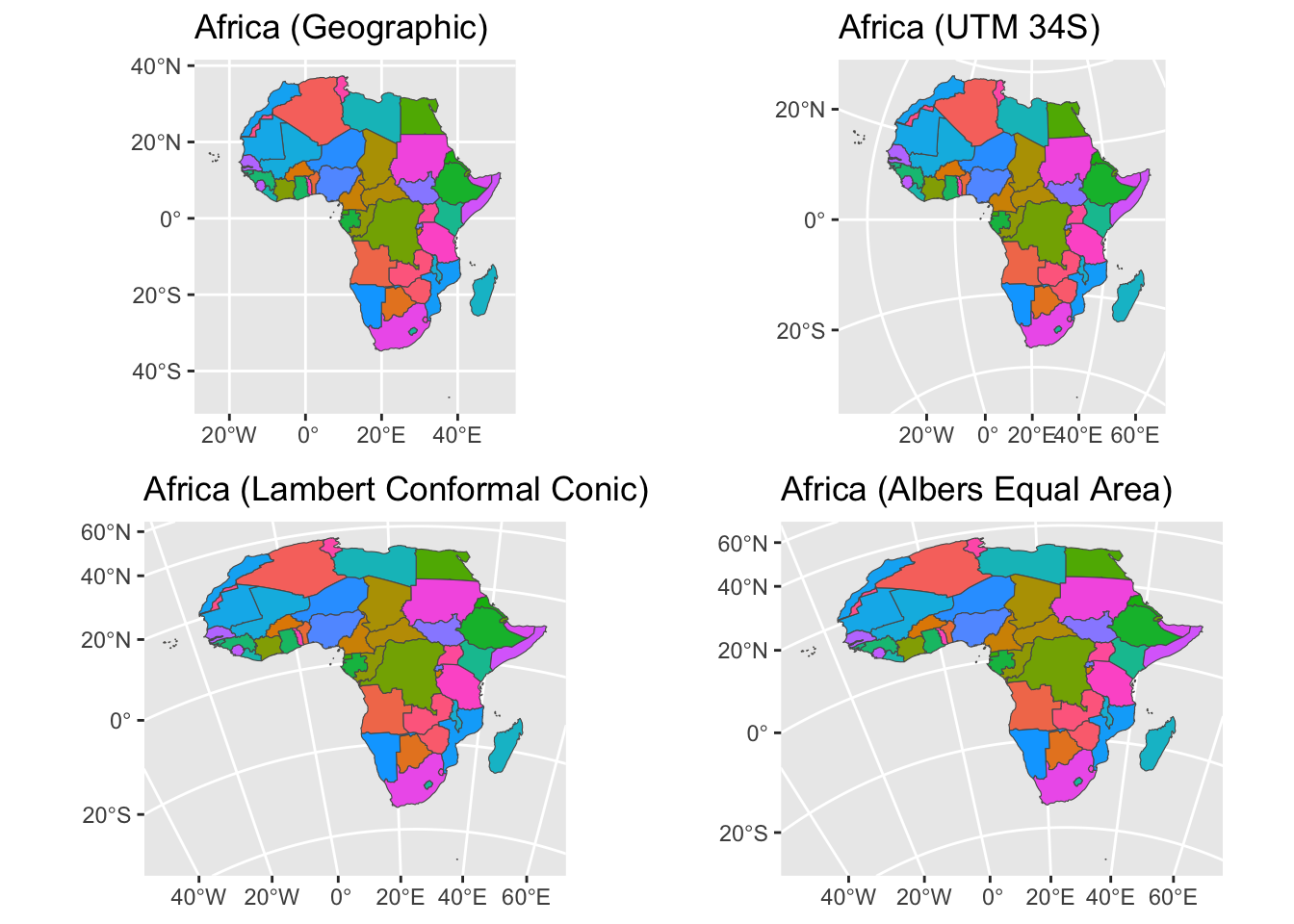
Figure 5.6: Africa, visualized with different coordinate reference systems. All four maps are different, even if the differences may be subtle!

5.2.4 “On the fly” vs manual projection

Note that some GIS tools can perform “on the fly” (re)projection of data. For example, by default ArcGIS sets the CRS for a project from the first dataset imported. When you want to visualize the data, it will reproject all other datasets to the set CRS so that it can visualize it properly. Similarly, ArcGIS and other software can project data in a geographic CRS to a projected CRS on the fly when asked to perform Euclidean measurement calculations.

On the fly projection can clearly be very useful, but it can also be misleading if you don’t know what its doing. This is especially problematic if it uses the wrong projection for the property you want to preserve!

You should always check the default settings for the software you’re using, and check the set CRS(s) and individual dataset CRS(s) to make sure you are working in a suitable CRS for the operations you want to perform!!!

5.2.5 The golden rules…

1. If things don’t line up, its probably a CRS issue.
2. You need to know what CRS your dataset is in.

• This is essential, because you need to define your projections to be able to compare datasets. If they are not the same, you will need to reproject one to align with the other*.
• If your datasets are not in the same CRS, most GIS software will give you warning or error messages, but not always! Note that not all file formats store the CRS “metadata”, so check and store it yourself if needed!

3. You need to make sure you use a CRS that best preserves the properties you are interested in (area, distance, direction, shape). More on this in section 5.2.2.
4. If your areas and distances are stupidly small (0.001 etc) your data are probably in Geographic (i.e. degrees and not a unit of distance like metres).
5. Always interrogate and “common-sense-check” your results!!!

*Defining Projection is not the same as reprojecting! Think in terms of languages, “I have text in Japanese and want it in English”. Defining is saying what it IS (“This text is in Japanese” - defining Japanese as English gives you garbage). Reprojecting is what you want it to be (i.e. translate Japanese to English).

Two other issues to look out for:

• The official South African CRS is waiting to get you. If you see Gauss Conform run screaming, its a left handed CRS based on Southings and Westings (i.e. completely inverted…). Simple, yes?
• Datums… These are essentially models of the shape of the surface of the planet. Most South African datasets (since 1999 at least) use the Hartebeesthoek 94 datum, which is our local “bespoke” solution. It’s pretty much the same as the WGS84 datum (a good global datum), and the difference is negligible for most ecological analyses. Our former local “bespoke” datum (the Cape or Clarke1880 datum), which was often used for data before 1999, is out to get you. These datasets will never line up perfectly with modern data sets when reprojected in a normal GIS and will usually be a couple of tens of metres off…

Some other important pitfalls to avoid are best covered in this chapter in Manny Gimond’s Intro to GIS and Spatial Analysis.