- A quick note on the structure of this tutorial
- Data Description
- Housekeeping
- Getting and cleaning the data, but first and foremost, projection!!!
- Let’s start with point data
- Raster data (mostly functions from library(raster))
- Polygons!
- Going parallel!!!
- Animation!
- Some other data visualization and analysis
- But what about our poor cedars?
- Options for writing out spatial data
This post follows on from Handling Spatial Data in R - #1. Getting started, which gives the basics on installing R and RStudio, CRAN Spatial Task Views and useful DIY resources. Obviously, if you’re already familiar with these topics then no need to go through that post. You may also be interested in the next post on handling big spatial data and memory management.
Here we’ll work through a practical example exploring fire history layers (polygon), topographic (raster) and locality (point) data using the libraries ‘rgdal’, ‘raster’ and ‘sp’ and a few others. The example will cover setting and changing projections and extents, subseting polygons, raster calculations, rasterizing polygons and extracting data with a few neat tricks and visualisations along the way. Note that you can navigate to and/or bookmark the various sections using the links in the table of contents above.
A quick note on the structure of this tutorial
From here this tutorial will include embedded chunks of R code and the output that R returns in little grey boxes. The R code I call starts at the beginning of the line, while each line of R’s output starts with “##”, e.g.
1+1## [1] 2Note that I occassionally include additional comments in the R chunks as one often does in normal R code. Comments are preceded by “#”, e.g.
1+1 #My comment## [1] 2Hopefully this will all make sense as you get into the tutorial…
Data Description
For this exercise we’ll play with fine-scale locality (point) data for the critically endangered Clanwilliam cedar (Widdringtonia cedarbergensis) mapped by my father for the Hike the Cederberg map (check out http://www.slingsbymaps.com/; data for 1000 trees downloadable here, a 90m (raster) digital elevation model (DEM) here (I will also show you how to download the DEM directly with R using the raster package), and two “polygon” data sets consisting of mapped burn scars for CapeNature reserves (available from SANBI’s BGIS website here and the National Vegetation Map (available here).
You will need to download the cedar dataset into your chosen local data directory (see datwd under “Housekeeping” below) and download the other data into your chosen GIS data directory (see giswd below) and unzip them. datwd and giswd can be the same for the purposes of this tutorial. You can download the R code (with the RMarkdown content commented out) at here.
Housekeeping
Apologies, this bit is a little long-winded, but please read it carefully as it will likely affect your ability to run the code below.
Working directories
I usually work from a “Project” in RStudio linked to a GIT repository (see https://git-scm.com/ and https://github.com/) for version control and easy code sharing/collaboration. I’m not going to go there with this tutorial, but it is worth exploring if you intend to do big projects in R. R projects set the working directory to a good place automatically. Alternatively you can use the setwd() function. If I’m not in a repo or I am working with large data sets that I don’t want to replicate in every GIT repo on my hard drive I usually set separate “data”, “GIS data” (i.e. biggish data) and “results” working directories by making each path an object and inserting as appropriate for different read and write functions using paste() or paste0(). These would look something like:
datwd = “/home/jasper/Dropbox/SAEON/Training/SpatialDataPrimer/Example/Data/”
giswd = “/home/jasper/Documents/GIS/”
reswd = “/home/jasper/Dropbox/SAEON/Training/SpatialDataPrimer/Example/Results/”
A quick aside on slashes
Often the reason you can’t read in data is because you need to add (or delete) a “/” at the end! - Silly, but that pro tip should help.
Note that we generally use single forwardslashes “/” in R. Windows likes to use single backslashes, but R (and just about every other computer programme in the world) doesn’t like this. You can use double backslashes on Windows if you must…
Libraries/packages
Here we call the extention libraries with functions we’ll need for this session. More on what R libraries/packages are in my previous post here.
You should install the libraries before running the code below using install.packages() while connected to the internet - e.g. install.packages(“raster”). Note that one occasionally encounters issues installing doMC, but you can usually install it from their development page using install.packages(“doMC”, repos=“http://R-Forge.R-project.org”). If neither of these work for you don’t worry, it is not an essential component of the tutorial.
library(raster, quietly = T) # To handle rasters
library(rasterVis, quietly = T) # For fancy raster visualisations
library(rgdal, quietly = T) # To communicate with GDAL and handle shape files
## rgdal: version: 1.4-4, (SVN revision 833)
## Geospatial Data Abstraction Library extensions to R successfully loaded
## Loaded GDAL runtime: GDAL 2.2.3, released 2017/11/20
## Path to GDAL shared files: /usr/share/gdal/2.2
## GDAL binary built with GEOS: TRUE
## Loaded PROJ.4 runtime: Rel. 4.9.3, 15 August 2016, [PJ_VERSION: 493]
## Path to PROJ.4 shared files: (autodetected)
## Linking to sp version: 1.3-1library(sp, quietly = T) # To handle shapefiles
library(doMC, quietly = T) # To run code in parallel
library(animation, quietly = T) # To make fancy animations...
library(dismo, quietly = T) # For fancy tricks in Google Earth
suppressPackageStartupMessages(library(googleVis, quietly = T)) # For even more fancy tricks in Google Earth## Creating a generic function for 'toJSON' from package 'jsonlite' in package 'googleVis'R should have give you a bunch of feedback after calling the libraries. Look out for errors or warnings suggesting that the packages aren’t installed properly. You can often ignore warnings, but it is useful to take note of them in case you encounter confusing problems later on.
Getting and cleaning the data, but first and foremost, projection!!!
R typically uses the PROJ.4 conventions for cartographic projections (or coordinate reference systems - CRS). Check out http://proj4js.org or http://spatialreference.org/ or google for the “proj4string” for various coordinate reference systems.
NOTE!!! Many R functions will allow you to play with objects with different CRS resulting in GARBAGE! Others will reproject one or other of the objects for you, but this can be slow and it’s not worth taking the chance. I recommend checking and setting your CRS for all objects. You can check CRS with proj4string(), check that multiple objects have the same CRS using identicalCRS(), and reproject objects of class “Spatial” with spTransform() and objects of class “Raster” with projectRaster(). Note that not all reprojections are possible or sensible, but I’ll leave that homework to you. One key case where reprojection in R appears to work (but doesn’t!) is reprojecting MODIS satellite data from its native Sinusoidal projection. My workaround is to use the gdalwarp() function in library(gdalUtils) - a very powerful set of functions which I explore in the next post on big spatial data and memory management.
I like to set a standardized CRS as an object that I can call throughout my workflow.
#Set a standardized projection using the PROJ.4 string convention
stdCRS <- "+proj=utm +zone=34 +south +ellps=WGS84 +datum=WGS84 +units=m +no_defs"

#This is also "EPSG:32734" - according to the European Petroleum Survey Group CRS convention - another common one
This is the Universal Transverse Mercator (UTM) projection, which is useful for studies with smallish extents (~<100km a side), because the unit is metres and is easily interpretable. The UTM zone we’re in for this example is 34 South http://whatutmzoneamiin.blogspot.co.za/p/map.html - so I’ve used UTM34S. More on projections for those interested here.
Let’s start with point data
Note!!! Here I’ll mostly use functions from library(rgdal) and library(sp). These have recently been superceded by library(sf), which covers functionality from these two packages and library(rgeos) and follows a Tidyverse approach to R coding. I’ve stuck with library(rgdal) and library(sp) because I first started this primer before library(sf) was released. I also feel its useful to see the diversity of ways in which things can be done in R (each have their pros and cons), and once you’ve learned it one way its easier to learn other ways. I hope to add a library(sf) tutorial (or section to this tutorial) at a later stage and will endeavour to add the link here ;) Note that library(sf) doesn’t deal with rasters so its still worth checking out the raster section of this post either way.
Reading in shapefiles
Ok, so lets use readOGR() from library(rgdal) to read the point data in as a shapefile. Note that readOGR() is incredibly versatile and can read in all kinds of shapefiles with different features (point, line, polygon) from different software - type ?rgdal for more info. Here R essentially calls the GDAL http://www.gdal.org/ software (the underpinning for QGIS and a number of other GIS software products). Unfortunately some PCs struggle to automatically install GDAL, but there are plenty of online fora providing solutions. Sometimes (although this issue may be fixed) there are conflicts between library(sp) and library(rgdal) depending on what order they are called.
rawpts <- readOGR(dsn=paste0(datwd, "Cedars.kml"), layer="Cedars.kml") # A Google Earth KML file## OGR data source with driver: LIBKML
## Source: "/home/jasper/Dropbox/SAEON/Training/SpatialDataPrimer/Example/Data/Cedars.kml", layer: "Cedars.kml"
## with 1000 features
## It has 11 fieldsproj4string(rawpts) # Check projection## [1] "+proj=longlat +datum=WGS84 +no_defs +ellps=WGS84 +towgs84=0,0,0"pts <- spTransform(rawpts, CRS(stdCRS)) # Do spatial transform to project to our chosen CRSNote the strange dsn=…, layer=… syntax. This will mess with you at first!!! This syntax is used to allow the function to read in many different file formats - type “ogrDrivers()” into the console to see a list. Different drivers often require different inputs for dsn= and layer=. I often have to play around or ask Google before I get it right for a new file type…
Also note the use of the paste0(datwd, “Cedars.kml”) trick I mentioned earlier:
paste0(datwd, "Cedars.kml")## [1] "/home/jasper/Dropbox/SAEON/Training/SpatialDataPrimer/Example/Data/Cedars.kml"Again, note that the presence and number of /’s are very important… It’s the first thing to check if you get an error!!! IF YOU HAVE ANY ISSUES READING IN DATA AT ANY STAGE THE FIRST THING TO DO IS TO RUN THE “paste0(…)” SECTION OF THE SCRIPT AND MAKE SURE IT MATCHES EXACTLY THE PATH TO YOUR FILE!!!
SpatialDataFrames
Let’s explore our point data a little more. Firstly, let’s look at the data class attribute.
class(pts)## [1] "SpatialPointsDataFrame"
## attr(,"package")
## [1] "sp"A “SpatialPointsDataFrame” - which is as it suggests - a set of spatial localities linked to a dataframe of information about each locality - like an attribute table in other GIS software. The nice thing is that R allows you to manipulate “Spatial(Point/Polygon/etc)Dataframes” in the same way as you can regular dataframes, e.g.
head(pts)## Name description timestamp begin end altitudeMode tessellate extrude
## 1 <NA> <NA> <NA> <NA> -1 0
## 2 <NA> <NA> <NA> <NA> -1 0
## 3 <NA> <NA> <NA> <NA> -1 0
## 4 <NA> <NA> <NA> <NA> -1 0
## 5 <NA> <NA> <NA> <NA> -1 0
## 6 <NA> <NA> <NA> <NA> -1 0
## visibility drawOrder icon
## 1 -1 NA <NA>
## 2 -1 NA <NA>
## 3 -1 NA <NA>
## 4 -1 NA <NA>
## 5 -1 NA <NA>
## 6 -1 NA <NA>Revealing that there’s not much in this object’s “attribute table”. Note that you can also subset using indexing [,], access columns using $, apply summary functions, etc as one does with a normal dataframe. We’ll do more of this in the Polygons section.
Accessing spatial coordinates and creating point shapefiles from spreadsheet data
We can easily extract the spatial coordinates from our object using coordinates().
head(coordinates(pts))## coords.x1 coords.x2
## [1,] 318630.2 6418166
## [2,] 329096.9 6411855
## [3,] 324656.3 6423442
## [4,] 324611.6 6427641
## [5,] 324156.0 6421462
## [6,] 320746.9 6429256These may look funny if you’re not familiar with UTM - the unit is metres, usually from the equator or poles and the Greenwich Meridian depending on the exact UTM CRS used.
We can also extract the coordinates and make them a regular “data.frame”" object (as if we’d read in a .txt or .csv file).
x <- as.data.frame(coordinates(pts))
class(x)
## [1] "data.frame"This allows me to demonstrate making a “Spatial” object by setting coordinates for x.
coordinates(x) <- ~ coords.x1 + coords.x2 #
class(x)
## [1] "SpatialPoints"
## attr(,"package")
## [1] "sp"As simple as that! But note that if you use this approach it will not have a coordinate reference system (the “proj4string”) and you have to assign it. Hopefully you know what CRS the geolocations were collected in!!!
str(x) # Note the lack of proj4string info## Formal class 'SpatialPoints' [package "sp"] with 3 slots
## ..@ coords : num [1:1000, 1:2] 318630 329097 324656 324612 324156 ...
## .. ..- attr(*, "dimnames")=List of 2
## .. .. ..$ : chr [1:1000] "1" "2" "3" "4" ...
## .. .. ..$ : chr [1:2] "coords.x1" "coords.x2"
## ..@ bbox : num [1:2, 1:2] 315518 6410827 333832 6434186
## .. ..- attr(*, "dimnames")=List of 2
## .. .. ..$ : chr [1:2] "coords.x1" "coords.x2"
## .. .. ..$ : chr [1:2] "min" "max"
## ..@ proj4string:Formal class 'CRS' [package "sp"] with 1 slot
## .. .. ..@ projargs: chr NAproj4string(x) <- stdCRS # To assign the CRS (IF IT IS KNOWN!!!)
str(x) # Note the presence of proj4string info## Formal class 'SpatialPoints' [package "sp"] with 3 slots
## ..@ coords : num [1:1000, 1:2] 318630 329097 324656 324612 324156 ...
## .. ..- attr(*, "dimnames")=List of 2
## .. .. ..$ : chr [1:1000] "1" "2" "3" "4" ...
## .. .. ..$ : chr [1:2] "coords.x1" "coords.x2"
## ..@ bbox : num [1:2, 1:2] 315518 6410827 333832 6434186
## .. ..- attr(*, "dimnames")=List of 2
## .. .. ..$ : chr [1:2] "coords.x1" "coords.x2"
## .. .. ..$ : chr [1:2] "min" "max"
## ..@ proj4string:Formal class 'CRS' [package "sp"] with 1 slot
## .. .. ..@ projargs: chr "+proj=utm +zone=34 +south +ellps=WGS84 +datum=WGS84 +units=m +no_defs +towgs84=0,0,0"Lastly, its always good practice to remove objects from R’s memory if we won’t need them again… See next post on handling big spatial data and memory management for more on this.
rm(x)NOTE: Many spatial data objects use “slots” to store various components of the data (the “@” symbols revealed when we look at the data structure with the str() function). The slots can be accessed using “@” like you would “$” to call a variable from a dataframe or object from a list, but it is RECOMMENDED THAT YOU DO NOT DO THIS… The reason being that slots were designed so that the R package developers can change the way slots work to improve efficiency, handle new or different objects etc. If you write code that accesses slots directly it may break next time the libraries are updated. There are functions for accessing all slots (e.g. proj4string(), coordinates(), etc.) or you can simply use regular dataframe functionality.
Raster data (mostly functions from library(raster))
Let’s get a digital elevation model (DEM) from the SRTM90 (Shuttle Radar Topography Mission)* digital elevation database, match projection, and trim to the same extent as “pts”.
*Jarvis A., H.I. Reuter, A. Nelson, E. Guevara, 2008, Hole-filled seamless SRTM data V4, International Centre for Tropical Agriculture (CIAT), available from http://srtm.csi.cgiar.org
Reading in, reprojecting and cropping raster data
We can download the data directly with R using the function getData() (type ?getData for details), but this can be slow because it downloads a much bigger area than we need. To save time I’ve downloaded the data before and saved it locally with the “path =” setting. I’ve also provided you with a link to the subsetted data you need in the Data Description section of the post above. Here’s the code if you’re interested - hashed (#) out so R sees it as a comment and doesn’t run it.
#dem <- getData('SRTM', lon=19, lat=-32.5, path = paste0(giswd, "SRTM/")) # download data from CGIAR websiteInstead we’ll read the data in from the local source using the very versatile raster() function.
dem <- raster(paste0(giswd, "SRTM/srtm_ced.tif")) # read in data from local source - NOTE THAT YOU MAY NEED TO UNZIP THE FILE YOU DOWNLOADED in the Data Description section!!!
proj4string(dem)
## [1] "+proj=longlat +datum=WGS84 +no_defs +ellps=WGS84 +towgs84=0,0,0"This is not our chosen projection for this tutorial so we need to reproject.
dem <- projectRaster(dem, crs=CRS(stdCRS)) # note that we use a different function for raster data than for shapefiles (points or polygon) - this can take a while...
proj4string(dem)
## [1] "+proj=utm +zone=34 +south +ellps=WGS84 +datum=WGS84 +units=m +no_defs +towgs84=0,0,0"Now let’s look at the extent of the DEM relative to the cedar locality data.
extent(dem)## class : Extent
## xmin : 266615.1
## xmax : 382010.1
## ymin : 6353842
## ymax : 6491056extent(pts)## class : Extent
## xmin : 315517.9
## xmax : 333832.2
## ymin : 6410827
## ymax : 6434186Our DEM has a MUCH larger extent than our cedars of interest and we should crop it.
E <- extent(pts) + c(-900, 900, -900, 900) # The "+ c(...)" term adds a 900m buffer around the trees
dem <- crop(dem, E) # Crop DEM to the buffered extent
Let’s have a quick look at what we’re working with (using the basic plot functions).
plot(dem) #plot the digital elevation model
points(pts, pch=20, cex=.1) #add the cedar localities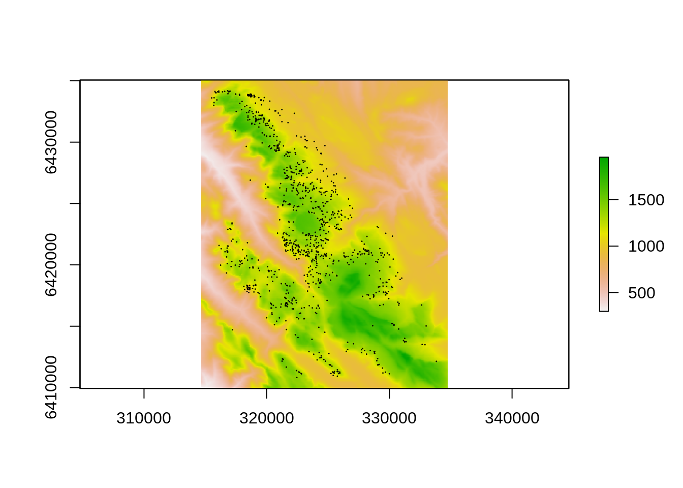
Calculating topographic information from a DEM
Now that we have the DEM cleaned up for our study let’s use the terrain() function to calculate/extract some topographic information. Note that terrain() is based on the more versatile focal() function, should you want to design your own indices etc. Also see rasterEngine() in library(spatial.tools) which is an equivalent, but with easy parallel processing capability.
slope <- terrain(dem, "slope")
aspect <- terrain(dem, "aspect")
TPI <- terrain(dem, "TPI") # Topographic Position Index
TRI <- terrain(dem, "TRI") # Terrain Ruggedness Index
roughness <- terrain(dem, "roughness")
flowdir <- terrain(dem, "flowdir")
But “aspect” is circular so small changes in the northern aspects (e.g. 2 to 358 degrees) look like big changes in the data. We can break aspect down into east-westness and north-southness using sin() and cos() - remember your trigonometry? (DISCLAIMER: This approach is not perfect and I’d recommend reading up about it if you intend to use it in your research).
eastwest <- sin(aspect)
northsouth <- cos(aspect)
Renaming and stack()ing rasters
Dealing with all these different rasters gets a bit cumbersome, but they have the same extent, resolution and grid so we can stack() them into one object. But first, we should make sure the data are named in a sensible way otherwise they can all end out being named “layer”…
names(eastwest)## [1] "layer"names(northsouth) ## [1] "layer"names(dem)## [1] "srtm_ced"names(eastwest) <- "eastwest" # To rename the data in the raster
names(northsouth) <- "northsouth"
names(dem) <- "dem"
topo <- stack(dem, slope, eastwest, northsouth, TPI, TRI, roughness, flowdir)
topo## class : RasterStack
## dimensions : 272, 256, 69632, 8 (nrow, ncol, ncell, nlayers)
## resolution : 78.5, 92.4 (x, y)
## extent : 314657.1, 334753.1, 6409929, 6435062 (xmin, xmax, ymin, ymax)
## crs : +proj=utm +zone=34 +south +ellps=WGS84 +datum=WGS84 +units=m +no_defs +towgs84=0,0,0
## names : dem, slope, eastwest, northsouth, tpi, tri, roughness, flowdir
## min values : 2.978850e+02, 7.817324e-05, -1.000000e+00, -1.000000e+00, -6.984706e+01, 4.181858e-01, 1.042966e+00, 1.000000e+00
## max values : 1957.903873, 1.114246, 1.000000, 1.000000, 90.148799, 139.760182, 436.692354, 128.000000# Another way to rename rasters in a stack
# names(topo) <- c("name1", "name2"", etc)Let’s look at what we’ve made.
plot(topo)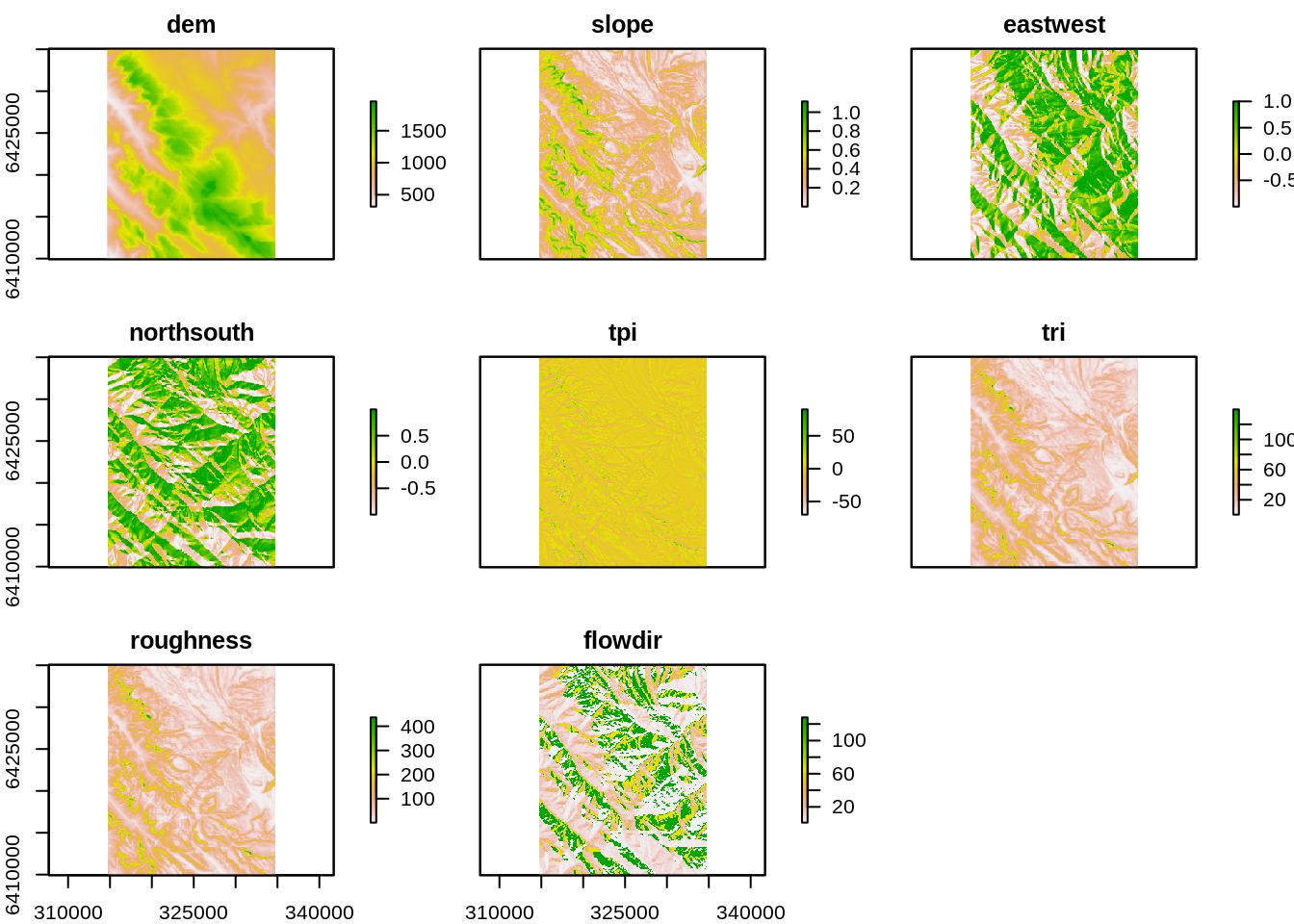
Rasterizing, aggregating and raster calculations
The raster library provides an amazing and very versatile environment for creating and working with rasters.
e.g. You easily can convert other data types into rasters using rasterize(), which allows you to specify the raster extent and resolution (or match an existing raster), and can apply functions so that you can chose what aspect of the data you’d like to focus on (e.g. the min, max or sum of a field in the attribute table of your vector layer). Here let’s rasterize the cedar points layer and calculate the tree density by 90m grid cell from the DEM.
dens <- rasterize(pts, dem, field="Name", fun="count")
plot(dens)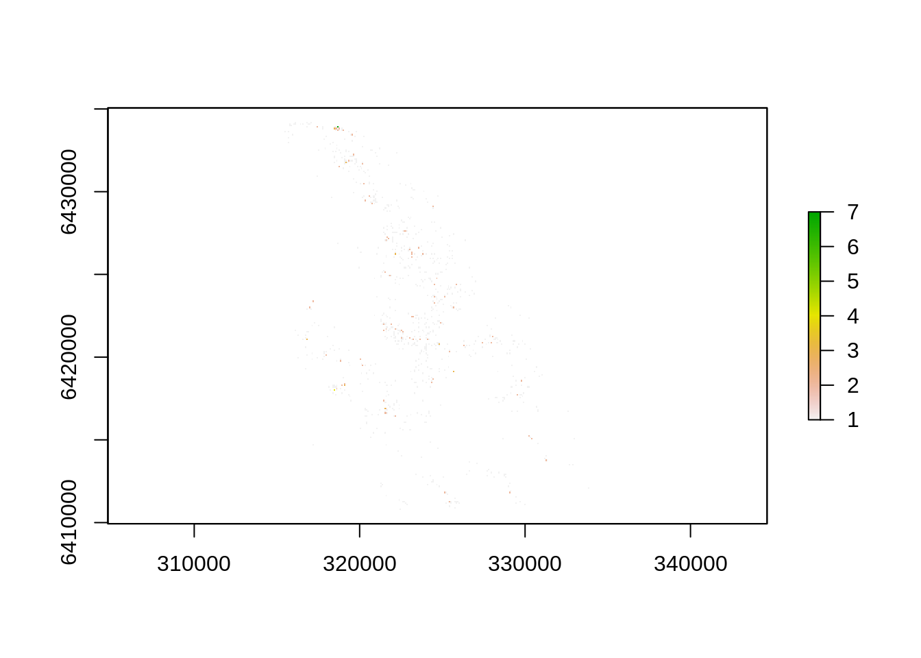
See anything? Probably not, these are 90m pixels in a large landscape… We can aggregate() the 90m pixels into larger units to make them more visible - e.g. 210m pixels by aggregating by a factor of three.
plot(aggregate(dens, fact=3, fun="sum"))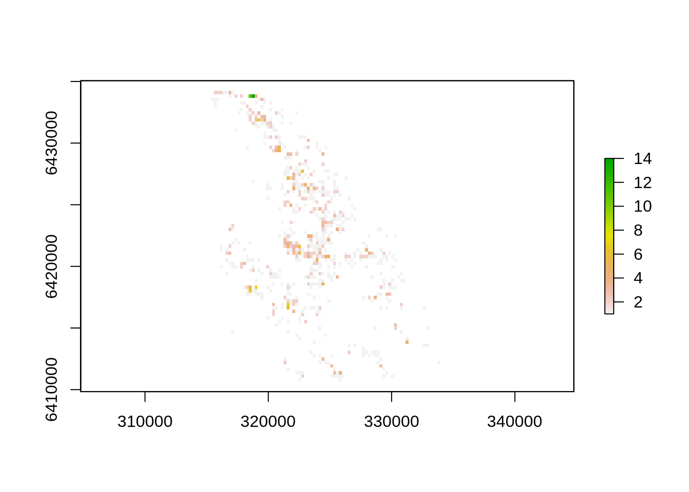
Better!
We can also apply raster calculations to only show the subset of cells with more than 10 trees - plotted in red to make it more visible.
plot(dens>10, col="red") # Use raster calculations to subset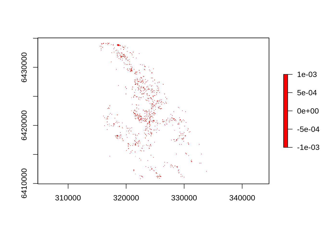
Note that you can add, subtract, multiply and divide rasters using code like raster1 + raster2 etc, which allows you to easily do some quite complicated calculations. Its also worth exploring the calc() function for designing and implementing more complicated functions.
Polygons!
Perhaps the best place to start is the National Vegetation Map of South Africa, Lesotho and Swaziland. Let’s get the data, set the CRS and crop to our area/extent of interest. Note that polygons, points and lines are all vector data (as opposed to raster) and you can handle them using the same functions.
vegmap <- readOGR(dsn=paste0(giswd, "VegMap/nvm2012beta2_wgs84_Geo"), layer="nvm2012beta2_wgs84_Geo") # Get the data## OGR data source with driver: ESRI Shapefile
## Source: "/home/jasper/Dropbox/BlogData/VegMap/nvm2012beta2_wgs84_Geo", layer: "nvm2012beta2_wgs84_Geo"
## with 44822 features
## It has 21 fieldshead(vegmap) # Have a look at the first 6 rows of the attribute table ## OBJECTID_1 NAME MAPCODE12 MPCDSUBT
## 0 0 Agulhas Limestone Fynbos FFl1 <NA>
## 1 1 Agulhas Limestone Fynbos FFl1 <NA>
## 2 2 Cape Seashore Vegetation AZd3 <NA>
## 3 3 Cape Seashore Vegetation AZd3 <NA>
## 4 4 Cape Seashore Vegetation AZd3 <NA>
## 5 5 Overberg Sandstone Fynbos FFs12 <NA>
## BIOREGION BIOME CHANGE_VER CHANGE_REF
## 0 South Coast Fynbos Bioregion Fynbos VM06 VegMap 2006
## 1 South Coast Fynbos Bioregion Fynbos VM06 VegMap 2006
## 2 Seashore Vegetation Azonal Vegetation VM06 VegMap 2006
## 3 Seashore Vegetation Azonal Vegetation VM06 VegMap 2006
## 4 Seashore Vegetation Azonal Vegetation VM06 VegMap 2006
## 5 Southwest Fynbos Bioregion Fynbos VM06 VegMap 2006
## CNSRV_TRGT SHAPE_LENG SHAPE_AREA BIOMECODE GRPCODE GROUP
## 0 32 5028.778 661226.69 F FFl Limestone Fynbos
## 1 32 25681.966 11720744.76 F FFl Limestone Fynbos
## 2 20 5624.948 332448.42 AZ AZd Seashore Vegetation
## 3 20 2241.355 73488.36 AZ AZd Seashore Vegetation
## 4 20 17366.045 1229468.26 AZ AZd Seashore Vegetation
## 5 30 1295.837 120756.02 F FFs Sandstone Fynbos
## BRGNCODE LEGEND VTYPSQKM12
## 0 F04 FFl 1 Agulhas Limestone Fynbos 294.4978
## 1 F04 FFl 1 Agulhas Limestone Fynbos 294.4978
## 2 AZd AZd 3 Cape Seashore Vegetation 243.5824
## 3 AZd AZd 3 Cape Seashore Vegetation 243.5824
## 4 AZd AZd 3 Cape Seashore Vegetation 243.5824
## 5 F02 FFs 12 Overberg Sandstone Fynbos 1169.4725
## DOCLINK SUBTYPENM BKSORT POLYSQKM
## 0 Descriptions\\FFl_1_2006.docx <NA> 01 11 001 0.6612
## 1 Descriptions\\FFl_1_2006.docx <NA> 01 11 001 11.7207
## 2 Descriptions\\AZd_3_2006.docx <NA> 10 02 003 0.3324
## 3 Descriptions\\AZd_3_2006.docx <NA> 10 02 003 0.0735
## 4 Descriptions\\AZd_3_2006.docx <NA> 10 02 003 1.2295
## 5 Descriptions\\FFs12_2006.docx <NA> 01 01 012 0.1208extent(vegmap) # Check the extent## class : Extent
## xmin : 16.45696
## xmax : 32.8914
## ymin : -34.8334
## ymax : -22.12583proj4string(vegmap) # Check the projection## [1] "+proj=longlat +datum=WGS84 +no_defs +ellps=WGS84 +towgs84=0,0,0"vegmap <- spTransform(vegmap, CRS(stdCRS)) # Reproject - This can take a while...
vegmap <- crop(vegmap, E) # Note that extent (E) was created earlier## Loading required namespace: rgeosNow let’s make a basic plot of what we’ve cropped…
cols <- rainbow(length(unique(vegmap$NAME))) # Make a set of 8 colours
plot(vegmap, col = cols[as.factor(as.character(vegmap$NAME))]) # Plot the map coloured by veg type
legend("bottomleft", legend = levels(as.factor(as.character(vegmap$NAME))), text.col = cols, cex=.6) # Add a legend
points(pts, pch=20, cex=.1) # Add the trees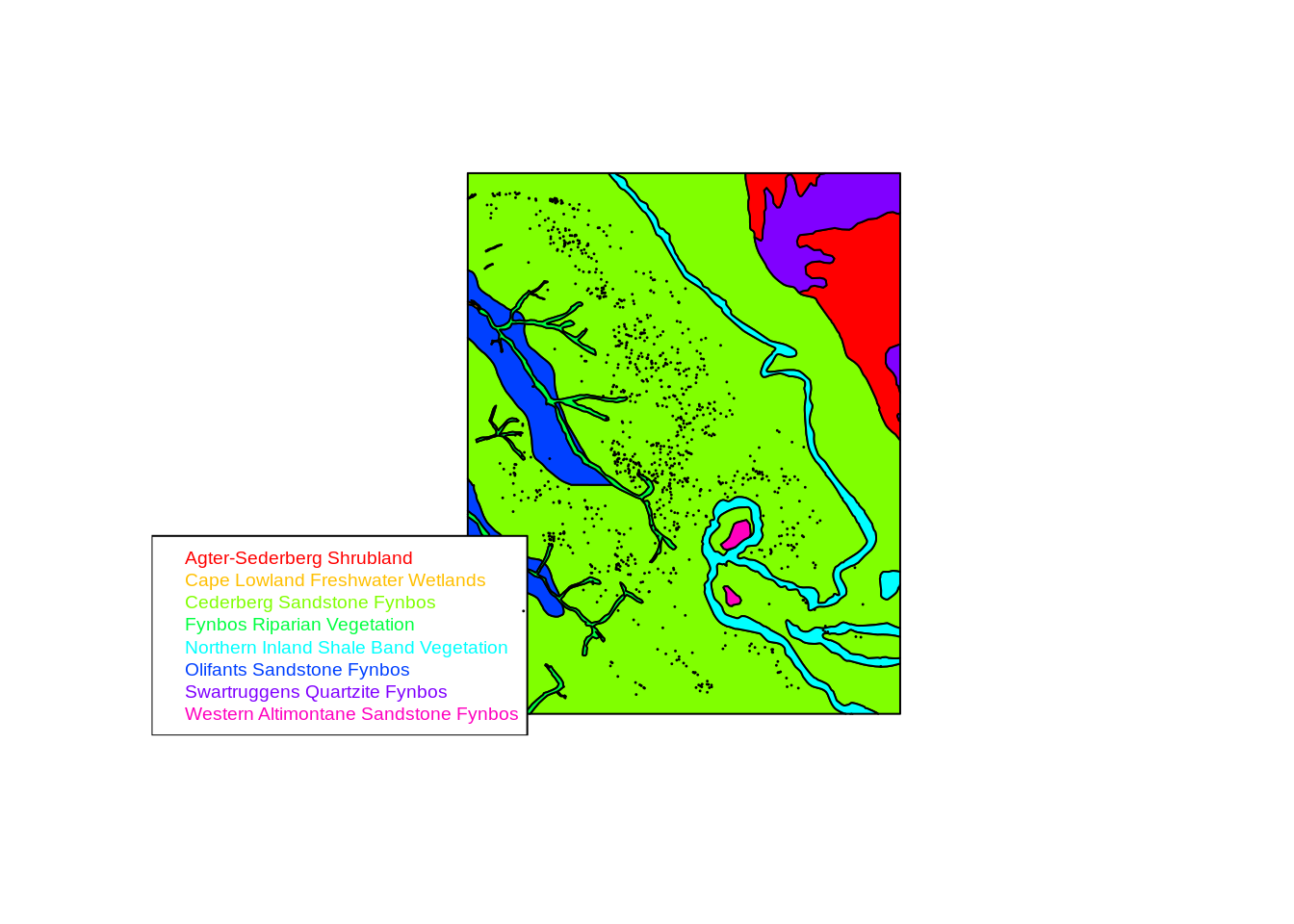
Looks like our cedars are restricted to “Cederberg Sandstone Fynbos”, but we can test that by extracting the veg type for each tree location. Note that there are a few ways of extracting data from spatial objects - we’ll use variants of the over() function for shapefiles.
treeveg <- over(pts, vegmap)
treeveg2 <- pts %over% vegmap
identical(treeveg, treeveg2)
## [1] TRUENote the two different approaches give the same result! Each have their own advantages depending on your style of coding, but I’ll leave it to you to find out more.
We’ve extracted the attribute table data for the vegtypes that each tree intersects into a new dataframe.
head(treeveg)## OBJECTID_1 NAME MAPCODE12 MPCDSUBT
## 1 7421 Cederberg Sandstone Fynbos FFs4 <NA>
## 2 7421 Cederberg Sandstone Fynbos FFs4 <NA>
## 3 7421 Cederberg Sandstone Fynbos FFs4 <NA>
## 4 7421 Cederberg Sandstone Fynbos FFs4 <NA>
## 5 7421 Cederberg Sandstone Fynbos FFs4 <NA>
## 6 7421 Cederberg Sandstone Fynbos FFs4 <NA>
## BIOREGION BIOME CHANGE_VER CHANGE_REF CNSRV_TRGT
## 1 Northwest Fynbos Bioregion Fynbos VM09 Helme (2007) WC 29
## 2 Northwest Fynbos Bioregion Fynbos VM09 Helme (2007) WC 29
## 3 Northwest Fynbos Bioregion Fynbos VM09 Helme (2007) WC 29
## 4 Northwest Fynbos Bioregion Fynbos VM09 Helme (2007) WC 29
## 5 Northwest Fynbos Bioregion Fynbos VM09 Helme (2007) WC 29
## 6 Northwest Fynbos Bioregion Fynbos VM09 Helme (2007) WC 29
## SHAPE_LENG SHAPE_AREA BIOMECODE GRPCODE GROUP BRGNCODE
## 1 1590266 2151887041 F FFs Sandstone Fynbos F01
## 2 1590266 2151887041 F FFs Sandstone Fynbos F01
## 3 1590266 2151887041 F FFs Sandstone Fynbos F01
## 4 1590266 2151887041 F FFs Sandstone Fynbos F01
## 5 1590266 2151887041 F FFs Sandstone Fynbos F01
## 6 1590266 2151887041 F FFs Sandstone Fynbos F01
## LEGEND VTYPSQKM12
## 1 FFs 4 Cederberg Sandstone Fynbos 2512.221
## 2 FFs 4 Cederberg Sandstone Fynbos 2512.221
## 3 FFs 4 Cederberg Sandstone Fynbos 2512.221
## 4 FFs 4 Cederberg Sandstone Fynbos 2512.221
## 5 FFs 4 Cederberg Sandstone Fynbos 2512.221
## 6 FFs 4 Cederberg Sandstone Fynbos 2512.221
## DOCLINK SUBTYPENM BKSORT POLYSQKM
## 1 Descriptions\\FFs_4_2006.docx <NA> 01 01 004 2151.887
## 2 Descriptions\\FFs_4_2006.docx <NA> 01 01 004 2151.887
## 3 Descriptions\\FFs_4_2006.docx <NA> 01 01 004 2151.887
## 4 Descriptions\\FFs_4_2006.docx <NA> 01 01 004 2151.887
## 5 Descriptions\\FFs_4_2006.docx <NA> 01 01 004 2151.887
## 6 Descriptions\\FFs_4_2006.docx <NA> 01 01 004 2151.887Now let’s look at the number of trees by veg type. Note the use of droplevels! If you don’t do this summary() will report all ~440 vegetation types in the country where cedars do not occur too… If you don’t know what I’m talking about you REALLY need to find out about factor levels - try this.
summary(droplevels(treeveg$NAME))## Cederberg Sandstone Fynbos
## 980
## Fynbos Riparian Vegetation
## 14
## Northern Inland Shale Band Vegetation
## 5
## Olifants Sandstone Fynbos
## 1So a few trees stray off Cederberg Sandstone Fynbos, but this could be errors in the veg mapping. Our vegmap is mostly mapped at 1:250 000 scale (i.e. ~2km error), while our tree locations are accurate to 10m…
Now let’s play with the CapeNature fire record data we downloaded earlier. Firstly, we get the data and transform to our standard CRS as for the vegmap.
firelayers <- readOGR(dsn=paste0(giswd, "CFR/All_fires_16_17_gw"), layer="All_fires_16_17_gw")## OGR data source with driver: ESRI Shapefile
## Source: "/home/jasper/Dropbox/BlogData/CFR/All_fires_16_17_gw", layer: "All_fires_16_17_gw"
## with 3842 features
## It has 16 fields
## Integer64 fields read as strings: idproj4string(firelayers)## [1] "+proj=longlat +datum=WGS84 +no_defs +ellps=WGS84 +towgs84=0,0,0"firelayers <- spTransform(firelayers, CRS(stdCRS))
extent(firelayers)## class : Extent
## xmin : 250253.7
## xmax : 733752.2
## ymin : 6150231
## ymax : 6453673Note that the fire data covers all CapeNature reserves across the CFR - I’ve done a quick and dirty exploration of patterns and trends for the whole region here for those interested. We could crop() to our extent (E), but there are other ways. Let’s explore and manipulate the data object a little. Note that the str() function is not useful when there are many layers (e.g. fires) - it just prints out all the details for each of the ~3500 separate fire layers… but calling the name of a spatial* object usually reports a summary and we can always explore the data as one does a dataframe.
firelayers## class : SpatialPolygonsDataFrame
## features : 3842
## extent : 250253.7, 733752.2, 6150231, 6453673 (xmin, xmax, ymin, ymax)
## crs : +proj=utm +zone=34 +south +ellps=WGS84 +datum=WGS84 +units=m +no_defs +towgs84=0,0,0
## variables : 16
## names : id, FIRE_CODE, Res_code, Region, Month, Year, Res_centre, Res_name, Local_desc, Datestart, Dateexting, Datewithd, Report_off, Police_Cas, Ignitionca, ...
## min values : 0, ANYS/00/1986/01, ANYS, Central, 0, 1927, Anysberg, Anysberg MCA, ?, 1927/05/28, 1940/06/27, 1944/01/16, ??, -, Fire operations - Block burns, ...
## max values : 9012, WBAY/12/2015/01, WBAY, Western, 12, 2017, Waterval, Zuurberg Nature Reserve, Zwartnek - west of Bergplaas, 2017/06/06, 7197/07/31, 2915/09/18, Zibele Blekiwe, yb285/11/2000, Unknown - Unknown, ...head(firelayers)## id FIRE_CODE Res_code Region Month Year Res_centre
## 0 0 OUTE/05/1927/01 OUTE Eastern 5 1927 Outeniqua
## 1 0 SWBG/12/1930/01 SWBG Eastern 12 1930 Swartberg
## 2 0 SWBG/01/1931/01 SWBG Eastern 1 1931 Swartberg
## 3 0 SWBG/08/1932/01 SWBG Eastern 8 1932 Swartberg
## 4 0 SWBG/02/1933/01 SWBG Eastern 2 1933 Swartberg
## 5 0 SWBG/02/1933/02 SWBG Eastern 2 1933 Swartberg
## Res_name Local_desc
## 0 Witfontein Nature Reserve 3322CD - 342
## 1 Groot Swartberg Nature Reserve Paardevley.3322BD.Fire no A1.
## 2 Groot Swartberg Nature Reserve De Wetsvley.3322AC.Fire no A2.
## 3 Groot Swartberg Nature Reserve Plaatberg.3321BD.Fire no.B1.
## 4 Grootswartberg MCA Blauwpunt.3322AD-BC.Fire no C1.
## 5 Groot Swartberg Nature Reserve Grootvlei.3321BD.Fire no.C2.
## Datestart Dateexting Datewithd Report_off Police_Cas
## 0 1927/05/28 <NA> <NA> <NA> <NA>
## 1 1930/12/28 <NA> <NA> <NA> <NA>
## 2 1931/01/18 <NA> <NA> <NA> <NA>
## 3 1932/08/17 <NA> <NA> <NA> <NA>
## 4 1933/02/11 <NA> <NA> <NA> <NA>
## 5 1933/02/11 <NA> <NA> <NA> <NA>
## Ignitionca Area_ha
## 0 Unknown - Unknown 3.852058
## 1 Natural - Lightning 172.562725
## 2 Natural - Lightning 198.357564
## 3 People - Farmer 2363.599963
## 4 Unknown - Unknown 5391.986432
## 5 Unknown - Unknown 2999.420641names(firelayers)## [1] "id" "FIRE_CODE" "Res_code" "Region" "Month"
## [6] "Year" "Res_centre" "Res_name" "Local_desc" "Datestart"
## [11] "Dateexting" "Datewithd" "Report_off" "Police_Cas" "Ignitionca"
## [16] "Area_ha"class(firelayers$Res_centre)## [1] "factor"levels(firelayers$Res_centre)## [1] "Anysberg" "Cederberg" "De Hoop"
## [4] "De Mond" "Driftsands" "Gamkaberg"
## [7] "Ganzekraal" "Geelkranz" "Goukamma"
## [10] "Grootvadersbosch" "Grootwinterhoek" "Hottentots-Holland"
## [13] "Jonkershoek" "Kammanassie" "Keurbooms"
## [16] "Kogelberg" "Limietberg" "Marloth"
## [19] "Matjiesrivier" "Outeniqua" "Riverlands"
## [22] "Robberg" "Swartberg" "Towerkop"
## [25] "Vrolijkheid" "Walker Bay" "Waterval"unique(firelayers$Res_centre)## [1] Outeniqua Swartberg Jonkershoek
## [4] Towerkop Gamkaberg Cederberg
## [7] Kammanassie Kogelberg Limietberg
## [10] Vrolijkheid Hottentots-Holland Grootvadersbosch
## [13] Marloth Grootwinterhoek Waterval
## [16] De Hoop Anysberg De Mond
## [19] Walker Bay Goukamma Riverlands
## [22] Keurbooms Robberg Driftsands
## [25] Ganzekraal Geelkranz Matjiesrivier
## 27 Levels: Anysberg Cederberg De Hoop De Mond Driftsands ... WatervalNote that we can subset shapefiles based on fields in the attribute table using indexing as one does with a regular dataframe. Each fire polygon is a separate row in the attribute table so we can extract all fires from the Cederberg by subsetting only the rows where the Res_centre = “Cederberg”.
firelayers <- firelayers[which(firelayers$Res_centre=="Cederberg"),]

firelayers$Res_centre <- droplevels(firelayers$Res_centre) # Remove unwanted factor levels that were passed on from the original full extent

levels(firelayers$Res_centre)
## [1] "Cederberg"plot(firelayers) # Plot (without colours)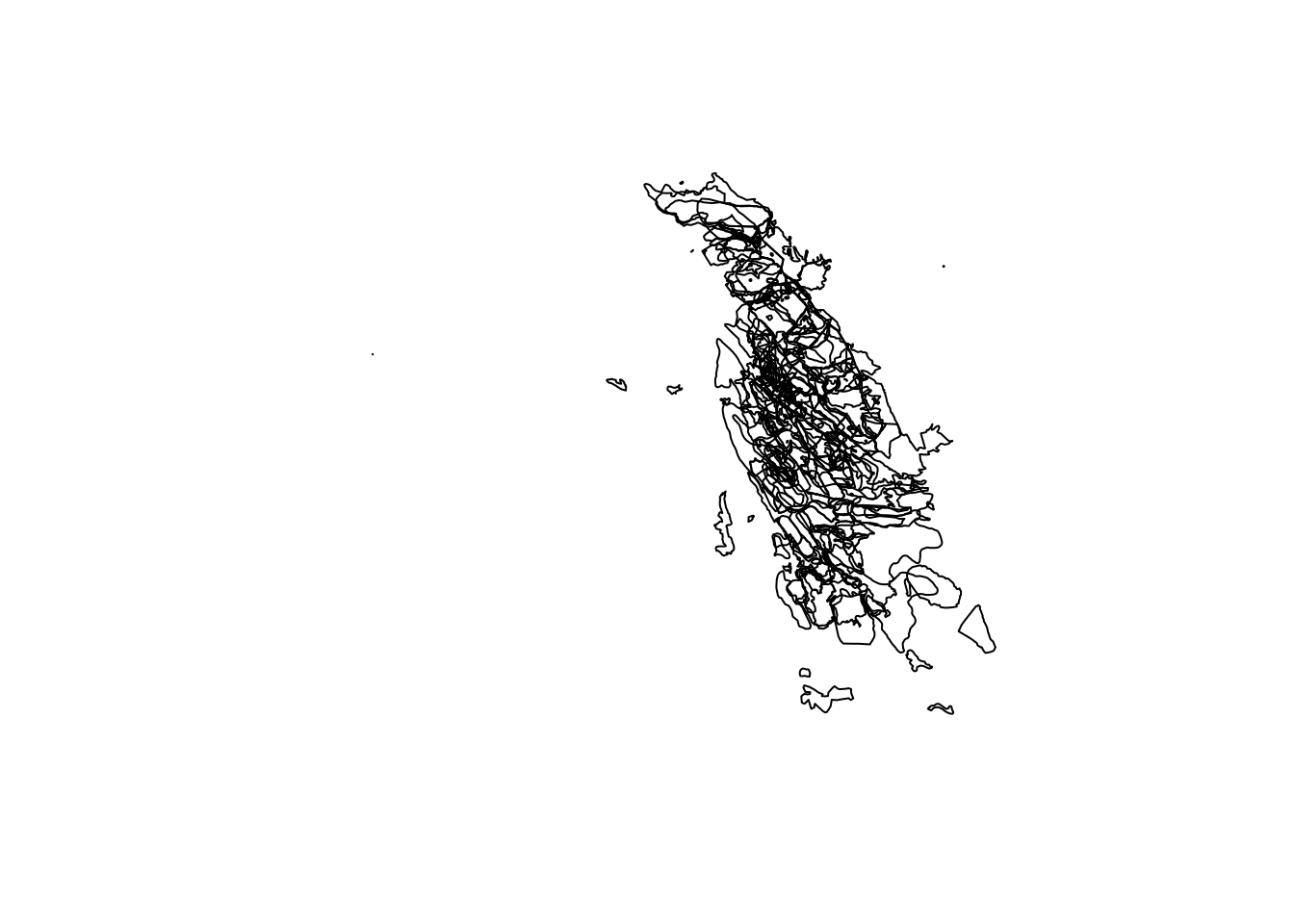
A cobweb? But vaguely the right shape to suggest its the Cederberg.
Let’s use rasterize() to create a raster of the number of fires in each 90m pixel of our digital elevation model, which may be prettier to plot. Since we want a raster of the count of fires per pixel we’ll set the function argument withing rasterize() to fun=“count”. Note that this requires a field/column with a unique value for each fire and we’re not sure if we have that, so we’ll create a new unique ID field “uID” and apply the function to that field.
firelayers$uID <- 1:nrow(firelayers) # Add an unique ID for each fire
firecount <- rasterize(firelayers, dem, field="uID", fun="count") # A count of all fires in each pixel
plot(firecount) # Note that the extent of our firelayers is larger than the DEM, but when rasterizing to an existing grid R trims it to the smaller extent automatically
points(pts, pch=20, cex=.1) # Add the trees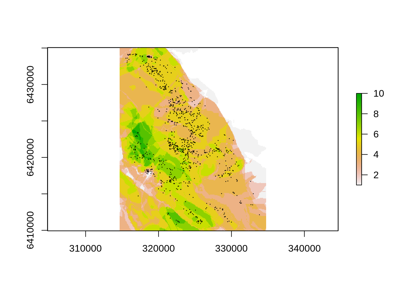
Now lets rasterize() each fire (date) into it’s own raster, but first we need to look at the underlying data and see if this will work…
names(firelayers)## [1] "id" "FIRE_CODE" "Res_code" "Region" "Month"
## [6] "Year" "Res_centre" "Res_name" "Local_desc" "Datestart"
## [11] "Dateexting" "Datewithd" "Report_off" "Police_Cas" "Ignitionca"
## [16] "Area_ha" "uID"firelayers$Datestart## [1] 1944/01/01 <NA> <NA> <NA> <NA> 1948/02/01
## [7] 1955/02/11 1956/04/15 1956/04/01 1958/03/29 1958/04/17 1958/04/18
## [13] 1958/05/01 <NA> <NA> <NA> <NA> 1959/02/09
## [19] 1959/03/23 1959/09/01 1959/10/01 1963/09/28 1963/01/10 1965/03/09
## [25] 1965/11/14 1965/01/29 1966/10/06 1967/03/11 1967/09/06 1967/12/29
## [31] <NA> 1968/09/13 <NA> 1969/03/22 1969/08/12 1969/09/29
## [37] 1969/09/29 1969/09/29 1969/09/29 1970/02/03 1970/02/05 2006/03/18
## [43] 2006/03/18 1970/04/21 1971/03/23 1971/07/20 <NA> 1972/03/11
## [49] <NA> 1972/05/01 1972/10/14 1972/12/07 1973/02/27 1973/02/27
## [55] 1973/04/24 1974/12/09 <NA> <NA> 1975/02/15 <NA>
## [61] 1975/11/26 1975/12/12 <NA> <NA> <NA> <NA>
## [67] 1976/01/30 1978/09/07 1978/09/18 1978/09/26 1978/10/05 1978/10/25
## [73] 1979/04/22 1979/08/06 1979/08/13 1979/08/14 1979/08/21 1979/08/24
## [79] 1979/12/25 1979/01/03 <NA> 1980/05/12 1980/05/29 1980/06/02
## [85] 1980/06/02 1980/06/02 1980/07/21 1980/08/14 1980/08/21 1980/08/25
## [91] 1981/02/20 1981/06/10 <NA> <NA> <NA> 1982/05/12
## [97] 1982/05/14 1982/05/14 1982/08/16 1982/08/17 1982/08/23 1982/08/25
## [103] 1982/09/22 1982/09/22 <NA> 1984/03/09 1984/03/22 1984/11/07
## [109] 1984/11/30 <NA> 1985/02/02 1985/02/02 1985/11/18 <NA>
## [115] 1986/12/14 1986/01/02 1986/01/14 1987/04/13 1987/04/03 1987/01/24
## [121] <NA> 1988/12/28 1988/12/28 1988/12/28 1988/12/28 1988/01/17
## [127] 1989/03/09 1989/04/26 1989/12/15 1989/01/15 1989/01/18 1990/05/25
## [133] <NA> 1991/04/30 1991/05/01 1991/05/12 1991/05/12 1991/05/12
## [139] 1991/05/12 1993/05/17 1993/05/17 1993/10/27 1993/01/13 1994/02/04
## [145] 1994/02/24 1995/05/23 1995/12/16 <NA> 1997/01/23 1998/02/15
## [151] 1998/03/05 1998/05/15 1998/05/15 1998/10/15 1998/10/19 1998/12/29
## [157] 1998/01/12 <NA> <NA> 1999/12/12 2000/10/11 <NA>
## [163] <NA> 2000/01/06 2001/03/06 2001/10/04 2002/02/24 2002/04/19
## [169] 2002/05/09 2002/12/06 2002/01/20 2002/01/01 2004/04/02 2004/09/21
## [175] 2004/12/22 2005/03/01 2005/10/11 2005/10/27 2005/11/09 2005/11/28
## [181] 2005/12/01 2006/02/06 2006/03/13 2006/03/28 2006/09/29 2006/12/05
## [187] 2006/12/23 2007/03/02 2007/03/02 2007/10/26 2007/01/19 2007/01/05
## [193] 2008/02/05 2008/02/07 2008/02/08 2008/01/12 2009/02/06 2009/03/11
## [199] 2009/12/10 2009/12/17 2010/02/10 2010/02/21 2011/02/18 2011/03/16
## [205] 2011/12/18 2011/01/31 2012/02/21 2012/02/22 2012/11/08 2012/11/20
## [211] 2012/12/14 2012/12/15 2012/12/21 2013/02/02 2013/02/02 2013/02/05
## [217] 2013/02/05 2013/03/11 2013/12/10 2013/12/20 2013/01/31 2013/01/25
## [223] 2013/01/25 2013/01/30 2013/01/16 2013/01/16 2014/02/13 2014/02/14
## [229] 2014/04/21 2014/07/22 2014/09/22 2014/12/19 2015/02/07 2015/02/20
## [235] 2015/02/21 2015/09/14 2015/09/14 2015/09/14 2015/09/14 2015/09/14
## [241] 2015/10/23 2015/11/21 2015/12/29 2016/03/05 2016/04/15 2016/04/19
## [247] 2016/05/23 2016/06/01 2016/09/09 2016/11/11 2016/12/15 2016/12/31
## [253] 2016/01/20 2016/01/17 2016/01/17 2016/01/09 2017/01/02
## 2540 Levels: 1927/05/28 1930/12/28 1931/01/18 1932/08/17 ... 2017/06/06What proportion of the “burnt area” recorded in the fire database does not have a start date?
sum(firelayers$Area_ha[is.na(firelayers$Datestart)])/sum(firelayers$Area_ha) ## [1] 0.07369786Oh dear, lets use “Year” instead…
firelayers$Year## [1] 1944 1945 1945 1945 1947 1948 1955 1956 1956 1958 1958 1958 1958 1958
## [15] 1958 1958 1958 1959 1959 1959 1959 1963 1963 1965 1965 1965 1966 1967
## [29] 1967 1967 1967 1968 1968 1969 1969 1969 1969 1969 1969 1970 1970 1970
## [43] 1970 1970 1971 1971 1971 1972 1972 1972 1972 1972 1973 1973 1973 1974
## [57] 1974 1974 1975 1975 1975 1975 1975 1975 1976 1976 1976 1978 1978 1978
## [71] 1978 1978 1979 1979 1979 1979 1979 1979 1979 1979 1979 1980 1980 1980
## [85] 1980 1980 1980 1980 1980 1980 1981 1981 1981 1981 1981 1982 1982 1982
## [99] 1982 1982 1982 1982 1982 1982 1982 1984 1984 1984 1984 1984 1985 1985
## [113] 1985 1985 1986 1986 1986 1987 1987 1987 1987 1988 1988 1988 1988 1988
## [127] 1989 1989 1989 1989 1989 1990 1990 1991 1991 1991 1991 1991 1991 1993
## [141] 1993 1993 1993 1994 1994 1995 1995 1995 1997 1998 1998 1998 1998 1998
## [155] 1998 1998 1998 1999 1999 1999 2000 2000 2000 2000 2001 2001 2002 2002
## [169] 2002 2002 2002 2002 2004 2004 2004 2005 2005 2005 2005 2005 2005 2006
## [183] 2006 2006 2006 2006 2006 2007 2007 2007 2007 2007 2008 2008 2008 2008
## [197] 2009 2009 2009 2009 2010 2010 2011 2011 2011 2011 2012 2012 2012 2012
## [211] 2012 2012 2012 2013 2013 2013 2013 2013 2013 2013 2013 2013 2013 2013
## [225] 2013 2013 2014 2014 2014 2014 2014 2014 2015 2015 2015 2015 2015 2015
## [239] 2015 2015 2015 2015 2015 2016 2016 2016 2016 2016 2016 2016 2016 2016
## [253] 2016 2016 2016 2016 2017Now we’re going to loop through our fire years and rasterize them one by one. There are some issues we need to address though:
Firstly, this may create a large object in R’s memory and slow it down. We can get around this by writing each raster out to a file. Geotif and some other formats allow writing multiple rasters to one file. We should also dump any unwanted objects from memory using rm().
Secondly, if there are a lot of cells in the raster and/or there are a lot of layers this operation may take some time either way. If we are on a multicore machine we can speed things up by parallelizing our code.
Thirdly, in this case we would like rasters for all years even if there were no fires (you’ll see why in a minute). We’ll use if() statements to identify years with no fires and fill these in with empty rasters (0’s only).
Lastly, if you end out running the code multiple times then you don’t want to have to repeat big operations like this. We can use file.exists() combined with an if() statement to only run this chunk of code if the file does not exist - see code below.
First let’s dump unwanted objects from memory and try rasterizing the fires on a single core using a normal for loop.
rm("aspect","slope", "eastwest", "northsouth", "TPI", "TRI", "roughness", "flowdir")

years <- min(firelayers$Year):max(firelayers$Year) # Get the unique list of years

rfifile <- paste0(datwd, "fires_annual_90m.tif") # Set a file name

system.time( # To time the process
if(!file.exists(rfifile)) { # Check if the file exists. If not, run this
td <- list() # Create an empty list
# Loop through years making a raster of burnt cells (1/0) for each
  for (i in 1:length(years)) {
  y <- years[i] # The index year
  # If no fires that year, return a raster of zeros
  if(sum(firelayers$Year==y)==0)
      td[[i]] <-  raster(extent(dem),res=res(dem),vals=0)
  # If there are fires, rasterize
  if(sum(firelayers$Year==y)>0)
      td[[i]] <- rasterize(firelayers[which(firelayers$Year==y),],dem, field="Year", fun="count", background=0)
  } # End loop
rfi <- stack(td)
writeRaster(rfi,file=rfifile) # Write out rasters to one file
} # End if() statement
) # End timing
## user system elapsed
## 0.000 0.000 0.001Note that you’ll see it takes 0 seconds on my machine - that’s because the statement if(!file.exists(rfifile)) on my machine is TRUE (i.e. I’d already made the output geotif before), so none of that code ran. You should see something different the first time you run it.
Going parallel!!!
Now lets try it in parallel using the foreach/%dopar% loop in library(doMC)… This is just one of many ways of setting up parallel processing in R, and not necessarily the best. I’ve just used it because foreach() is an easy extention of a for() loop. There are many options!!! For a quick primer have a look at this blog post.
First, we need to set the machine up for parallel processing by registering the cores we want to use as a cluster. We’ll autodetect the number of cores on your machine (using detectCores()) and use one less - allowing you to still work on other programmes on your machine while the code runs
registerDoMC(detectCores()-1)Now let’s set an output file name and run the code in parallel with the foreach() function.
rfifileP <- paste0(datwd, "fires_annual_90m_parallel.tif") # Set a file name

system.time( # To time the process
if(!file.exists(rfifileP)) { # Check if the file exists. If not, run this
# Start parallel processing
rfi <- foreach(y=years,.combine=stack,.packages="raster") %dopar% {
 # Loop through years making a raster of burnt cells (1/0) for each
  # Check if there were any fires that year, if not, return zeros
  if(sum(firelayers$Year==y)==0)
      td <-  raster(extent(dem),res=res(dem),vals=0)
  # If there are fires, rasterize
  if(sum(firelayers$Year==y)>0)
      td <- rasterize(firelayers[which(firelayers$Year==y),],dem, field="Year", fun="count", background=0)
  # Return the individual raster
  return(td)
  } # End parallelized code
writeRaster(rfi,file=rfifileP) # Write out the set of rasters to one file
} # End if() statement
) # End timing
## user system elapsed
## 0.000 0.000 0.001There shouldn’t be much time difference on your machine in this case, but then this is a small example and most of the time is spent interpreting the input code rather than processing. Going parallel really pays when crunching big analyses…
Now lets read in the layers we wrote out and plot them.
rfi <- stack(rfifile) # Read the files back in as a stack
rfi # Look at the stack
## class : RasterStack
## dimensions : 272, 257, 69904, 74 (nrow, ncol, ncell, nlayers)
## resolution : 78.3, 92.4 (x, y)
## extent : 314587.6, 334710.7, 6409924, 6435056 (xmin, xmax, ymin, ymax)
## crs : +proj=utm +zone=34 +south +datum=WGS84 +units=m +no_defs +ellps=WGS84 +towgs84=0,0,0
## names : fires_annual_90m.1, fires_annual_90m.2, fires_annual_90m.3, fires_annual_90m.4, fires_annual_90m.5, fires_annual_90m.6, fires_annual_90m.7, fires_annual_90m.8, fires_annual_90m.9, fires_annual_90m.10, fires_annual_90m.11, fires_annual_90m.12, fires_annual_90m.13, fires_annual_90m.14, fires_annual_90m.15, ...names(rfi)=paste0("Fire_",years) # Add year as name for each raster
rfi <- crop(rfi, E) # Crop to just our area of interest (speeds things up)
plot(rfi) # Plot all layers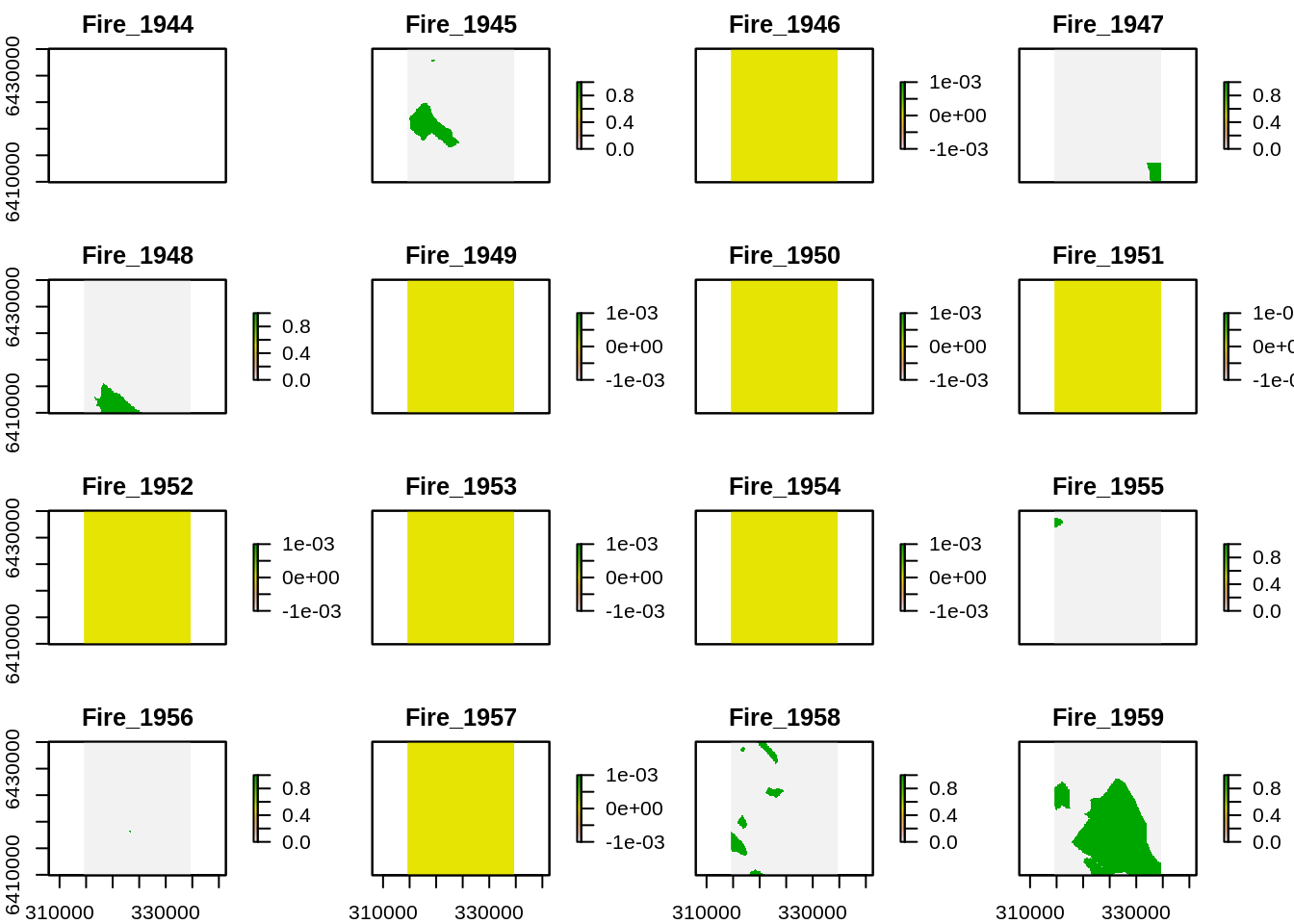
Pretty messy… there must be a sexier way?
Animation!
There are more and more ways of producing cool animations and interactive graphics in R. Here’s a simple example using library(animation). Note that this reqires installing the stand-alone software http://www.imagemagick.org/.
if(!file.exists(paste0(reswd,"fires.gif"))) { # Check if the file exists
  saveGIF({
    for (i in 1:dim(rfi)[3]) plot(rfi[[i]],
                      main=names(rfi)[i],
                      legend.lab="Fire!",
                      col=rev(terrain.colors(2)),
                      breaks=c(-0.1,.1,1.1))},
    movie.name = paste0(reswd,"fires.gif"),
    ani.width = 480, ani.height = 600,
    interval=.5)
}
Hmm… not that impressive… What if we take advantage of raster calculations and add all the rasters leading up to each time step using sum()?
if(!file.exists(paste0(reswd,"firesadded.gif"))) { # Check if the file exists
  saveGIF({
    for (i in 1:dim(rfi)[3]) plot(sum(rfi[[1:i]], na.rm=T), #Note the summing of rasters 1 to i
                      main=names(rfi)[i],
                      legend.lab="Fire!",
                      col=rev(terrain.colors(11)),
                      breaks=c(seq(-0.5,10.5,1)))},
    movie.name = paste0(reswd,"firesadded.gif"),
    ani.width = 480, ani.height = 600,
    interval=.5)
}
Much prettier!
Some other data visualization and analysis
# Plotting functions in library(rasterVis)
levelplot(dem)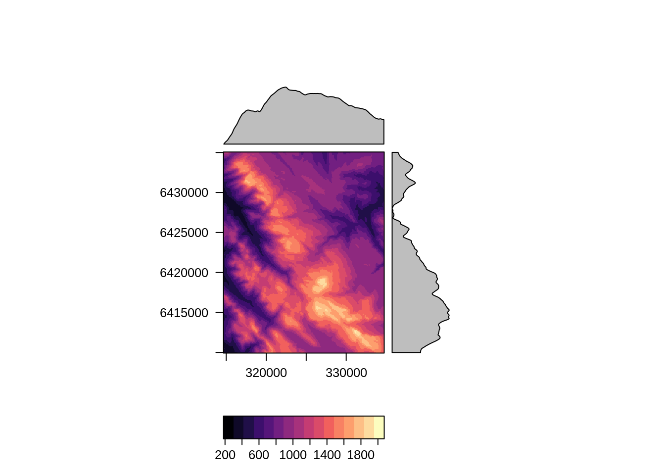
contourplot(dem)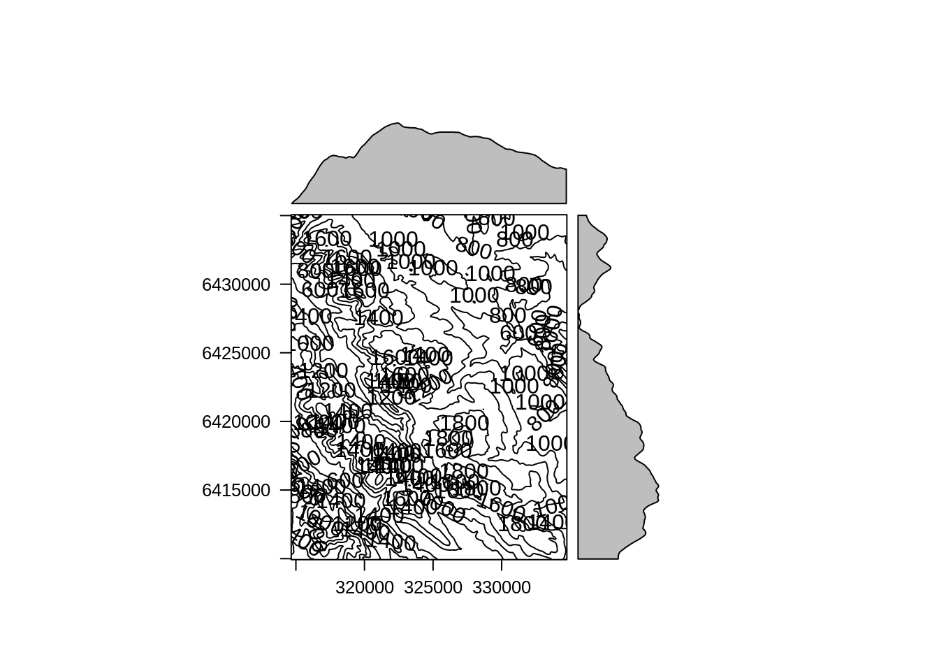
persp(dem)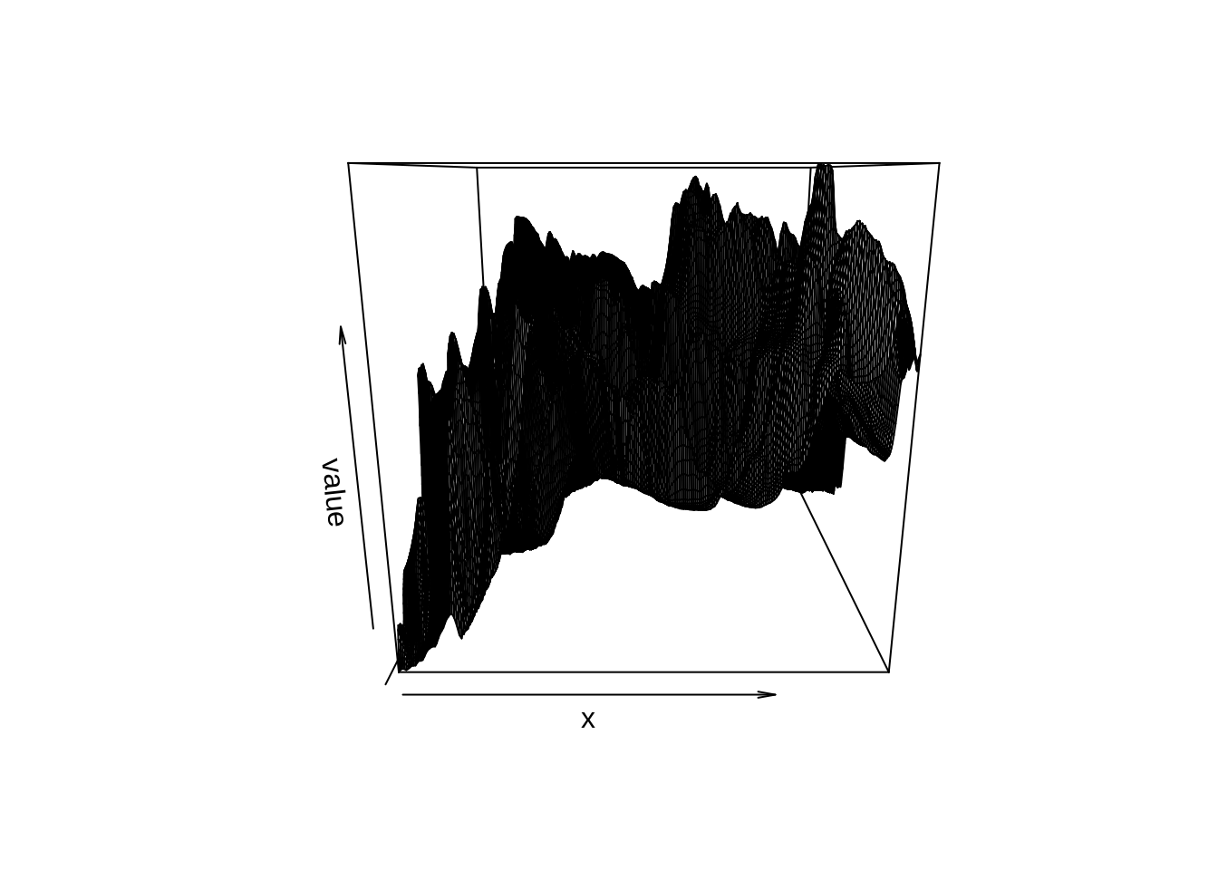
Some fancy tricks with Google Earth and library(googleVis)…
(Note that this only works for embedding into RMarkdown or an html page).
op <- options(gvis.plot.tag="chart") # Set gvis options for rmarkdown

points.gb <- as.data.frame(rawpts[sample(1:1000, 20),]) # Just select a few trees
points.gb$latlon <- paste(points.gb$coords.x2, points.gb$coords.x1, sep=":")
map.gb <- gvisMap(points.gb, locationvar="latlon", tipvar="Name")
plot(map.gb)
options(op) # Reset gvis options to defaultNote that you may get a “For development purposes only” or similar watermark. This is because Google Maps is no longer free - although it seems like their strategy is in flux. At one stage you needed to register with a credit card and get an API key. Google then allows $200 free usage per month (which is a lot!) before they start charging. This kind of visualization can also be done with Leaflet for R - for a demo from my work have a look at this post.
But what about our poor cedars?
I haven’t even shown you how to extract the topographic data from a raster!
This is easily done with extract()
topo$fire <- firecount #add the layer of numbers of fires
pts_topo <- extract(topo, pts) #extract data to a dataframe
head(pts_topo) #have a look
## dem slope eastwest northsouth tpi tri
## [1,] 1044.059 0.5108771 -0.8210832 -0.5708085 -3.8863532 35.66669
## [2,] 1235.577 0.6188006 -0.6050917 -0.7961558 -2.6656155 47.77104
## [3,] 1225.392 0.4177898 0.9581280 0.2863404 -21.6071677 30.67003
## [4,] 1011.958 0.1287723 0.9926773 -0.1207966 -13.7023358 15.55578
## [5,] 1229.284 0.4063195 0.1510045 -0.9885331 -5.8350988 31.47352
## [6,] 1415.163 0.5016256 0.9872718 0.1590420 0.7006943 33.74041
## roughness flowdir fire
## [1,] 133.16994 8 2
## [2,] 164.07892 8 4
## [3,] 113.06181 1 5
## [4,] 43.96513 1 2
## [5,] 88.13804 4 5
## [6,] 102.90161 1 5But there are multiple trees per 90m pixel, so some sites (pixels) are repeated. Perhaps this is better dealt with by including the tree density count raster.
topo$dens <- dens #add the tree density raster to the stack
dat = as.data.frame(topo) #check out ?rasterToPoints too

plot(dens ~ fire, data=dat)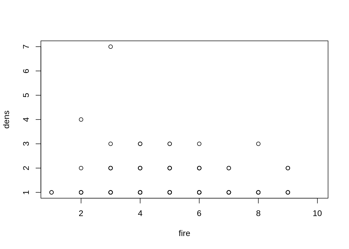
plot(dens ~ tri, data=dat)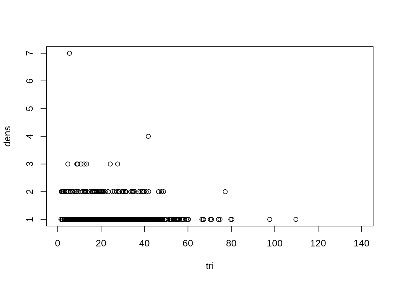
plot(dens ~ dem, data=dat)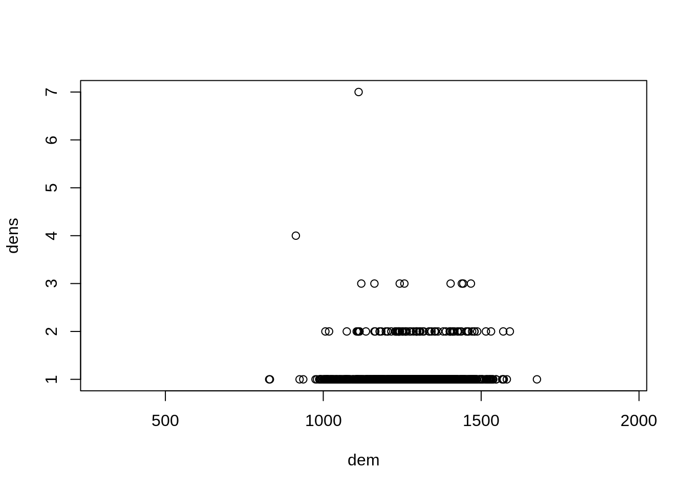
plot(dens ~ northsouth, data=dat)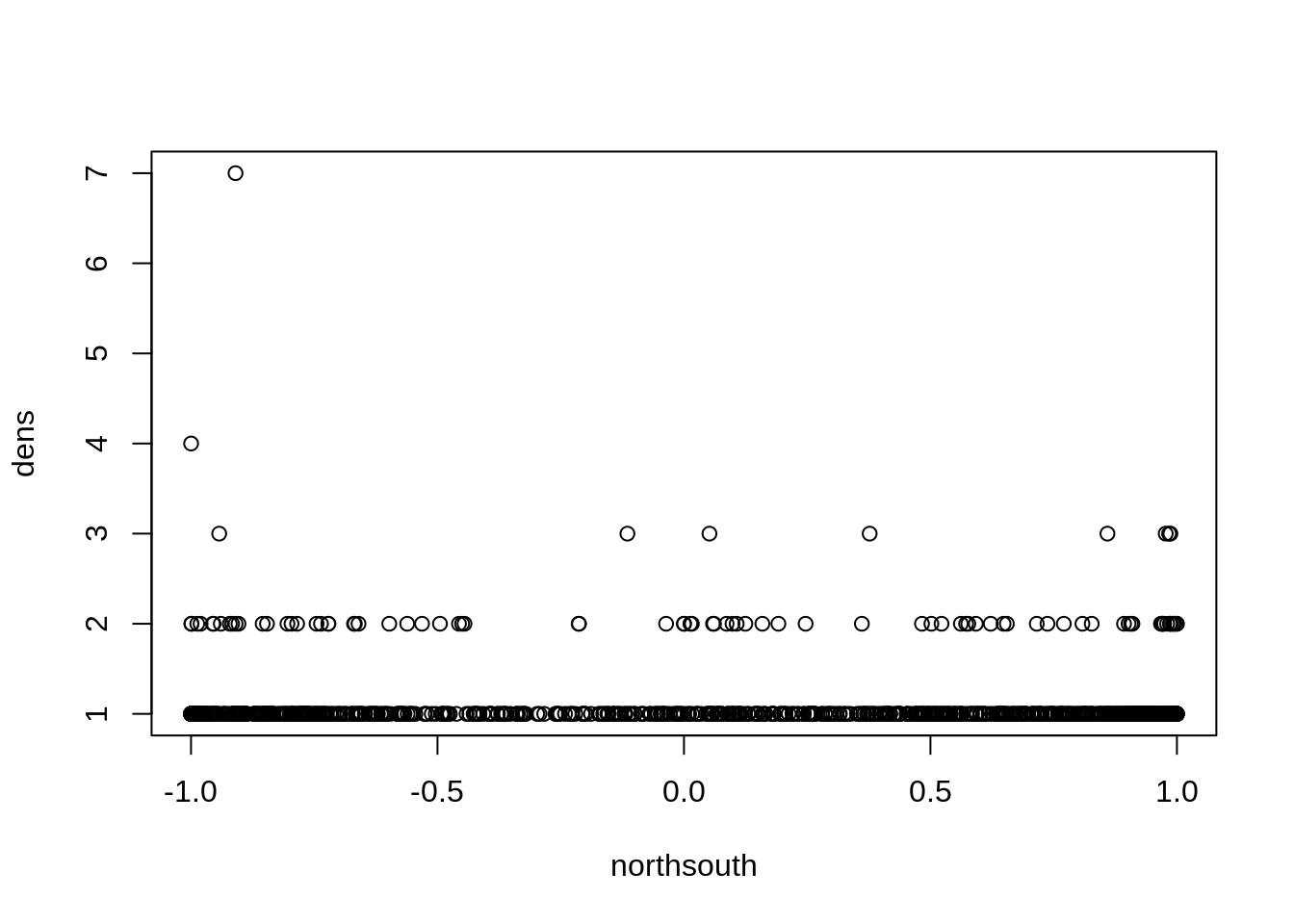
Current theories around the cedar’s decline include increased fire frequency and climate change. Here are a couple of basic hypotheses we could test:
Under increased fire frequency we would expect fewer cedars in areas where greater numbers of fires occur, but higher survival in areas with greater topographic roughness as this may provide refuge from fire (note that just the perimeters are mapped for most fires).
Under climate change we may expect cedars to be more numerous at higher altitudes, at more southern latitudes (although we don’t cover much latitudinal range here), and on South-facing slopes.
We can model the species’ distribution based on these variables using functions in the package dismo. Here I just do a quick BioClim model, but you can run many other models too. Even MaxEnt is available if you install it separately and tell R where it is on your machine.
bc <- bioclim(topo[[-10]], pts) # The [[-10]] tells R not to use the 10th raster (dens) in the model fitting as this would be circular...

p <- predict(topo, bc) # Predict potential distribution back onto base data
plot(p)
points(pts, pch=20, cex=.1)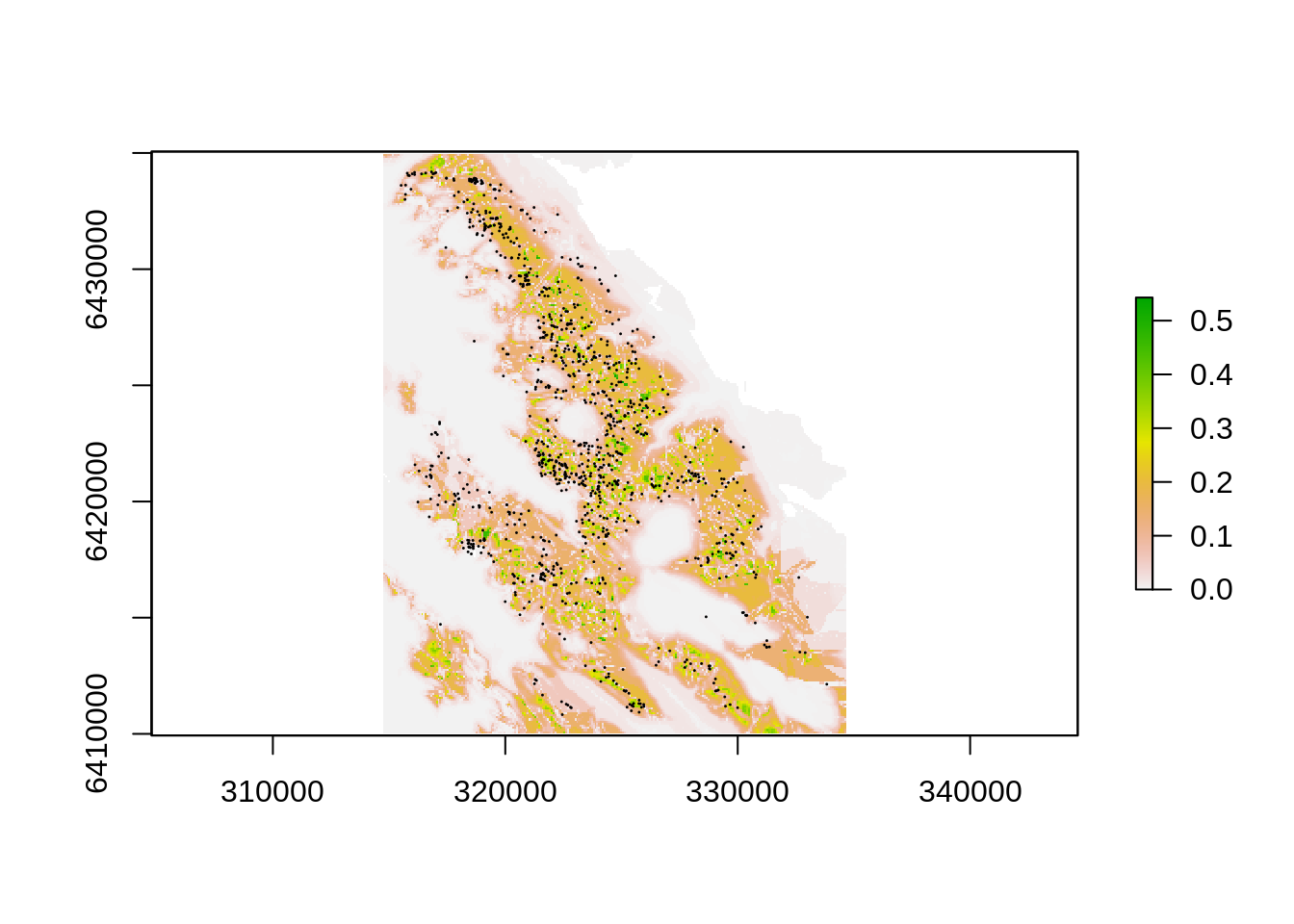
NOTE THAT I DO NOT EVALUATE THE MODEL IN ANY WAY - so I will not interpret it either. This is just a quick and dirty, breaking all the rules. Read up on species distribution modelling if you plan to use these techniques - the vignette on Species Distribution Modelling with R in library(dismo) is a good place to start. Type vignette(“sdm”) to call up the pdf.
Options for writing out spatial data
Here are a few useful functions, but also look for the “filename = …” or “outputfile = …” or similar options in the functions you use as these are often the most efficient.
?writeOGR # For shapefiles - can save in many many formats
?writeRaster # For rasters - also has many formats
?save # To write out a subset of objects from the project
?save.image # To write out the whole project with all objects (like a .mxd in ArcGIS really)
THANKS!!!
If you try this code and have issues the session info is below. Also note that all kinds of weird settings to Flash etc are required to do the gvisMap plot and it only works if embedded in an HTML webpage or similar. Feel free to leave a comment below - especially if you spot errors etc!
If you’re dealing with big spatial data files, you may be interested in the next post on big spatial data and memory management.
sessionInfo()## R version 3.6.1 (2019-07-05)
## Platform: x86_64-pc-linux-gnu (64-bit)
## Running under: Ubuntu 18.04.3 LTS
##
## Matrix products: default
## BLAS: /usr/lib/x86_64-linux-gnu/blas/libblas.so.3.7.1
## LAPACK: /usr/lib/x86_64-linux-gnu/lapack/liblapack.so.3.7.1
##
## locale:
## [1] LC_CTYPE=en_ZA.UTF-8 LC_NUMERIC=C
## [3] LC_TIME=en_ZA.UTF-8 LC_COLLATE=en_ZA.UTF-8
## [5] LC_MONETARY=en_ZA.UTF-8 LC_MESSAGES=en_ZA.UTF-8
## [7] LC_PAPER=en_ZA.UTF-8 LC_NAME=C
## [9] LC_ADDRESS=C LC_TELEPHONE=C
## [11] LC_MEASUREMENT=en_ZA.UTF-8 LC_IDENTIFICATION=C
##
## attached base packages:
## [1] parallel stats graphics grDevices utils datasets methods
## [8] base
##
## other attached packages:
## [1] googleVis_0.6.4 dismo_1.1-4 animation_2.6
## [4] doMC_1.3.6 iterators_1.0.10 foreach_1.4.4
## [7] rgdal_1.4-4 rasterVis_0.45 latticeExtra_0.6-28
## [10] RColorBrewer_1.1-2 lattice_0.20-38 raster_2.9-5
## [13] sp_1.3-1
##
## loaded via a namespace (and not attached):
## [1] Rcpp_1.0.1 knitr_1.23 magrittr_1.5
## [4] viridisLite_0.3.0 stringr_1.4.0 tools_3.6.1
## [7] grid_3.6.1 xfun_0.7 rgeos_0.4-3
## [10] htmltools_0.3.6 yaml_2.2.0 digest_0.6.19
## [13] bookdown_0.14 codetools_0.2-16 evaluate_0.14
## [16] rmarkdown_1.13 blogdown_0.16 stringi_1.4.3
## [19] compiler_3.6.1 jsonlite_1.6 hexbin_1.27.3
## [22] zoo_1.8-6## processing file: /home/jasper/GIT/jslingsbyblog/content/post/spatial-data-in-r-2-a-practical-example.Rmd## output file: /home/jasper/Dropbox/SAEON/Training/SpatialDataPrimer/Example/Data/PrimerSpatialData.R